Last update: 20230823
Table of contents
SetID for VSAT
When preparing a dataset for a Variant Set Association Test (VSAT) using SKAT (Sequence Kernel Association Test), it’s crucial to create a setID which lists the variants in a set (e.g. gene). This allows for collapsing SNPs into genes for gene-level analysis. The same is true for pathway sets, or any other virtual panel. The R package for SKAT, SKAT-O, etc. is https://github.com/leelabsg/SKAT.
1. Prepare plink format data
Convert from VCF to plink https://www.cog-genomics.org/plink2/. Here is an example plink.bim file: .bim (PLINK extended MAP file) https://www.cog-genomics.org/plink2/formats#bim.
| Chr | SNPID | Misc | Position | Allele 1 | Allele 2 |
|---|---|---|---|---|---|
| 1 | . | 0 | 10153 | G | A |
| 1 | . | 0 | 10159 | G | A |
| 1 | . | 0 | 10403 | * | ACCCTAACCCTAACCCTAACCCTAACCCTAACCCTAAC |
| 1 | . | 0 | 10403 | A | ACCCTAACCCTAACCCTAACCCTAACCCTAACCCTAAC |
| 1 | . | 0 | 10492 | T | C |
| 1 | . | 0 | 16068 | C | T |
| 1 | . | 0 | 16103 | G | T |
| 1 | . | 0 | 17385 | A | G |
| 1 | . | 0 | 17406 | T | C |
| 1 | . | 0 | 17407 | A | G |
Extended variant information file accompanying a .bed binary genotype table. (–make-just-bim can be used to update just this file.) A text file with no header line, and one line per variant with the following six fields:
- Chromosome code (either an integer, or ‘X’/’Y’/’XY’/’MT’; ‘0’ indicates unknown) or name
- Variant identifier
- Position in morgans or centimorgans (safe to use dummy value of ‘0’)
- Base-pair coordinate (1-based; limited to 231-2)
- Allele 1 (corresponding to clear bits in .bed; usually minor)
- Allele 2 (corresponding to set bits in .bed; usually major)
- Allele codes can contain more than one character. Variants with negative bp coordinates are ignored by PLINK.
Set SNP variant ID
We can set the missing variant IDs in a bim file with plink --set-missing-var-ids @_#\$r_\$a to give: 1_10153_G_A in the .bim SNPID column.
2. Downloading Ensembl mart data
The first step involves acquiring gene position data. This will let one map SNPs to specific genes. This data is downloaded from the Ensembl BioMart: http://mart.ensembl.org/biomart/martview.
- Data Acquired: Gene stable ID, start and end positions, chromosome/scaffold name, and additional annotations like gene names and MIM morbid descriptions.
Source: Ensembl BioMart, providing comprehensive and up-to-date gene information corresponding to the GRCh38.p14 assembly of the human genome.
- Example output of mart.tsv:
| Gene stable ID | Gene start (bp) | Gene end (bp) | Chromosome/scaffold name | Gene name | MIM morbid description |
|---|---|---|---|---|---|
| ENSG00000210049 | 577 | 647 | MT | MT-TF | |
| ENSG00000211459 | 648 | 1601 | MT | MT-RNR1 | |
| ENSG00000210077 | 1602 | 1670 | MT | MT-TV | |
| ENSG00000210082 | 1671 | 3229 | MT | MT-RNR2 | |
| ENSG00000209082 | 3230 | 3304 | MT | MT-TL1 | |
| ENSG00000198888 | 3307 | 4262 | MT | MT-ND1 | LEBER OPTIC ATROPHY;;LEBER HEREDITARY OPTIC NEUROPATHY; LHON |
| ENSG00000198888 | 3307 | 4262 | MT | MT-ND1 | MITOCHONDRIAL MYOPATHY, ENCEPHALOPATHY, LACTIC ACIDOSIS, AND STROKE-LIKE EPISODES; MELAS;;MELAS SYNDROME |
| ENSG00000210100 | 4263 | 4331 | MT | MT-TI | |
| ENSG00000210107 | 4329 | 4400 | MT | MT-TQ | |
| ENSG00000210112 | 4402 | 4469 | MT | MT-TM |
You can also get this via R biomaRt:
# Install and load the biomaRt package
if (!requireNamespace("biomaRt", quietly = TRUE)) {
    install.packages("BiocManager")
    BiocManager::install("biomaRt")
}
library(biomaRt)
2. Preparing the File.SetID
The file format for SKAT SetID is described in the package documentation https://cran.r-project.org/web//packages/SKAT/SKAT.pdf. Using the downloaded Ensembl Mart data, the File.SetID is prepared. This file is critical as it establishes a relationship between SNPs in the dataset and their respective genes:
- Integration of SNP Data: The BIM file from a PLINK dataset is utilized, where SNPs are annotated with chromosome and position data.
- Mapping SNPs to Genes: The BIM data (SNP data) is merged with the Ensembl Mart data. This involves filtering and aligning SNPs to their corresponding gene based on the chromosome and positional data.
- Output: A SetID file that lists each SNP under its respective gene, facilitating the collapsing of SNPs for gene-level analysis in SKAT.
The SetID file is a white-space (space or tab) delimitered file with 2 columns: SetID and SNP_ID. Please keep in mind that there should be no header! The SNP_IDs and SetIDs should be less than 50 characters, otherwise, it will return an error message.
- Example File.SetID
| SNPID | SetID |
|---|---|
| 1_10153_G_A | Gene1 |
| 1_10159_G_A | Gene1 |
| 1_16068_C_T | Gene2 |
| 1_16103_G_T | Gene2 |
3. Running SKAT for a VSAT Per Gene
After preparing the SetID file, SKAT is executed to assess the association of gene-level variants (collapsed SNPs) with the phenotype of interest. Here’s a simplified explanation of how SKAT is run for VSAT per gene:
- Input Files: Besides the SetID file, necessary inputs include BED, BIM, and FAM files that provide the genotype and family data.
- SetID File: It defines SNP sets where each set corresponds to a gene, and SNPs within each set are those mapped to the gene.
- Kernel Choice and Adjustment: SKAT uses kernel-based methods to assess the aggregate effect of multiple SNPs. Choices of kernel can affect the sensitivity and specificity of the results, especially in the context of different genetic architectures.
- Statistical Framework: SKAT employs a variance-component score test framework. This framework accommodates various types of complex genetic models, including those with multiple causal variants of varying effect sizes.
Technical Details
SKAT provides various options to fine-tune the analysis:
- Kernels: Options include linear, linear.weighted, and others, each suitable for different scenarios and hypotheses about genetic effects.
- Weighting Schemes: Influence the emphasis on rare vs. common variants, often based on minor allele frequencies.
- Imputation of Missing Data: Methods like fixed, bestguess, or random can handle missing genotypes, crucial for maintaining robustness in genetic data analysis.
- Phenotypic Adjustments: Continuous or dichotomous phenotypes are supported, with options to adjust for covariates and complex sample structures.
By preparing the dataset and understanding the intricacies of SKAT, you can effectively conduct VSAT to screen for an enriched set (.e.g. gene or pathway) by running one SKAT-O test per setID.
Interpretation of VSAT with Archipelago plot
You might use our Archipelago package to illustrate the results of complex VSAT studies https://github.com/DylanLawless/archipelago. This can be used to combine variant-level GWAS with gene-level, pathway-level, or other variant set tests.
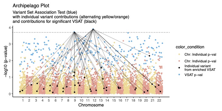
“Summary and illustration of variant set association test statistics. Variant set association tests (VSAT), particularly those incorporating minor allele frequency variants, have become invaluable in genetic association studies by allowing robust statistical analysis with variant collapse. Unlike single variant tests, VSAT statistics cannot be assigned to a genomic coordinate for visual interpretation by default. To address these challenges, we introduce the Archipelago plot, a graphical method for interpreting both VSAT p-values and individual variant contributions. The Archipelago method assigns a meaningful genomic coordinate to the VSAT p-value, enabling its simultaneous visualization alongside individual variant p-values. This results in an intuitive and rich illustration akin to an archipelago of clustered islands, enhancing the understanding of both collective and individual impacts of variants. The Archipelago plot is applicable in any genetic association study that uses variant collapse to evaluate both individual variants and variant sets, and its customizability facilitates clear communication of complex genetic data. By integrating two dimensions of genetic data into a single visualization, VSAT results can be easily read and aid in identification of potential causal variants in variant sets such as protein pathways.”