Bayesian: Part 2 Probability of a girl birth given placenta previa
Last update:
## [1] "2024-11-29"
This doc was built with: rmarkdown::render("Bayesian_example2.Rmd", output_file = "../pages/bayesian_example2.md")
Introduction to part 2
The code is based on a version by Aki Vehtari.
In the continuation of the analysis on placenta previa, we look at different priors to understand their impact on the posterior distribution. This part not only revisits the basic steps introduced in Part 1 but also expands on them by exploring alternative prior settings to illustrate the sensitivity of our posterior estimates to the choice of prior.
Following the initial setup where we determined the posterior distribution using a uniform prior, Part 2 investigates how different priors influence the results. This is crucial for assessing the robustness of our conclusions against the assumptions we make in our Bayesian framework.
- \(X = 437\) - number of female births in placenta previa
- \(Y = 543\) - number of male births in placenta previa
- \(n = 980\) - total births in placenta previa
- \(0.485\) - the frequency of normal female births in the population
- As in part 1, we had a posterior Beta(438,544)
a <- 437 # girls
b <- 543 # boys
Exploring the effect of different priors
Density evaluation: We calculate the density of the posterior distribution over a range of theta values using a uniform prior for simplicity.
# Evaluate densities at evenly spaced points between 0.375 and 0.525
df1 <- data.frame(theta = seq(0.375, 0.525, 0.001))

# Posterior with Beta(1,1), ie. uniform prior
df1$pu <- dbeta(df1$theta, a+1, b+1)
Further prior variations: We set up priors with varying strengths by modifying the prior counts and success ratio, reflecting different degrees of confidence in the prior information.
# 3 different choices for priors
# Beta(0.485*2,(1-0.485)*2)
# Beta(0.485*20,(1-0.485)*20)
# Beta(0.485*200,(1-0.485)*200)
n <- c(2, 20, 200) # prior counts
apr <- 0.485 # prior ratio of success
- Beta distribution parameters: These parameters are set to reflect increasing confidence in prior information, with the product of 0.485 and multipliers (2, 20, 200) determining the strength of the prior belief. This adjustment in parameters influences how much the prior beliefs affect the Bayesian updating process.
- Prior counts (
n): Specifies the strength of the prior. Lower counts like 2 suggest minimal prior influence, while higher counts like 200 indicate a strong prior belief based on substantial evidence or confidence. - Prior probability of success (
apr): Represents an assumed rate of female births, serving as the basis for setting the Beta distribution parameters, thereby impacting the shape of the posterior distribution.
This setup allows for the examination of how prior beliefs, quantified by n and apr, impact the posterior estimates. By varying these priors, we see the Bayesian framework’s sensitivity to initial assumptions, highlighting the need for careful consideration of prior information in Bayesian analysis.
The following helper function and lapply construct compile the dataset as described: helperf computes prior and posterior densities for a range of theta values based on varying strengths of prior beliefs. This is combined using lapply across different prior settings, and the results are consolidated and reshaped for plotting
# helperf returns for given number of prior observations, prior ratio
# of successes, number of observed successes and failures and a data
# frame with values of theta, a new data frame with prior and posterior
# values evaluated at points theta.
helperf <- function(n, apr, a, b, df)
  cbind(df, pr = dbeta(df$theta, n*apr, n*(1-apr)), po = dbeta(df$theta, n*apr + a, n*(1-apr) + b), n = n)

# lapply function over prior counts n and pivot results into key-value pairs.
df2 <- lapply(n, helperf, apr, a, b, df1) %>%
  do.call(rbind, args = .) %>%
  pivot_longer(!c(theta, n), names_to = "density_group", values_to = "p") %>%
  mutate(density_group = factor(density_group, labels=c('Posterior','Prior','Posterior with unif prior')))

# add correct labels for plotting
df2$title <- factor(paste0('alpha/(alpha+beta)=0.485, alpha+beta=',df2$n))
# Plot distributions
ggplot(data = df2) +
  geom_line(aes(theta, p, color = density_group)) +
      # proportion of girl babies in general population
  geom_vline(xintercept = pop_freq, linetype='dotted') +
  annotate(geom = "label", label = lab_pop, x = pop_freq, y = 20, hjust = 0, fill = "white",  alpha = 0.5, size =2) +
  facet_wrap(~title, ncol = 1)
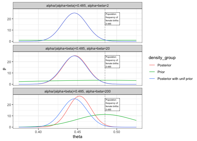
The resulting plots highlight how the choice of prior affects the posterior, with visual cues like vertical lines at the prior mean and faceting by scenario.
Conclusion
The exploration in part 2 demonstrates the Bayesian framework’s flexibility and the critical role of prior selection. By comparing different priors, we see how prior beliefs can substantially influence posterior outcomes, thereby affecting conclusions drawn from Bayesian analysis.