Understanding the role and features of PCA in genetic analysis
Last update: 20250106
PCA in genomic analysis
For example of PCA correcting for population structure in GWAS see https://cloufield.github.io/GWASTutorial/05_PCA/.
Haplotype blocks
Consider how DNA is inherited from parents: during recombination, each chromosome in the nucleus - whether autosomal (chr1-22), sex (X, Y), or mitochondrial (Mt) - receives one DNA strand from each parent. These strands then break and exchange segments, resulting in a mix of parental DNA in the offspring, yet maintaining two copies of each chromosome.
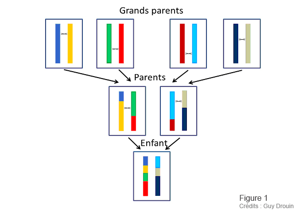
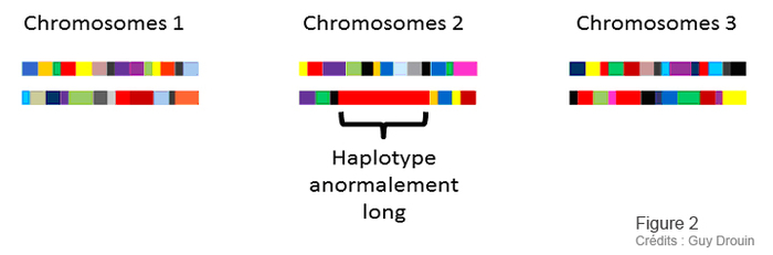
Figure 1 and 2: Guy Drouin, Université d’Ottawa, for ACFAS.ca magazine.
As illustrated in Figure 1, each generation sees a number of “crossings” between our various heritages, at different points. In this way, the intact or “non-recombining” pieces - the famous haplotypes - become smaller and smaller with each generation. For example, figure 2 shows that the second copy of chromosome 2 contains an abnormally long haplotype. It is therefore a much more recent piece of chromosome than the others. In fact, this abnormally long haplotype represents a piece of chromosome that contains a useful variant. It enabled the person with this variant to survive better, and this person passed this variant on to his or her descendants. The more favorable a variant, the faster it spreads through the population.
Haplotype blocks and genetic analysis
This recombination process creates long stretches of DNA, known as haplotype blocks, which are identical to those found in one parent or the other. By identifying a variant in a parent, one can track the same genetic block in the child, which will include the variant. This approach underlies methods like cheap genotyping and genome-wide association studies (GWAS), which focus on these blocks rather than individual genetic variants.
The Function of PCA
As human populations have migrated and diversified, these haplotype blocks have mixed differently across regions, reflecting historical patterns of human movement. Principal Component Analysis (PCA) captures these differences in haplotype block distributions, correlating them with ancestral geographic origins. This is crucial for adjusting genetic studies for population stratification, ensuring that associations found are due to genetics and not population bias.
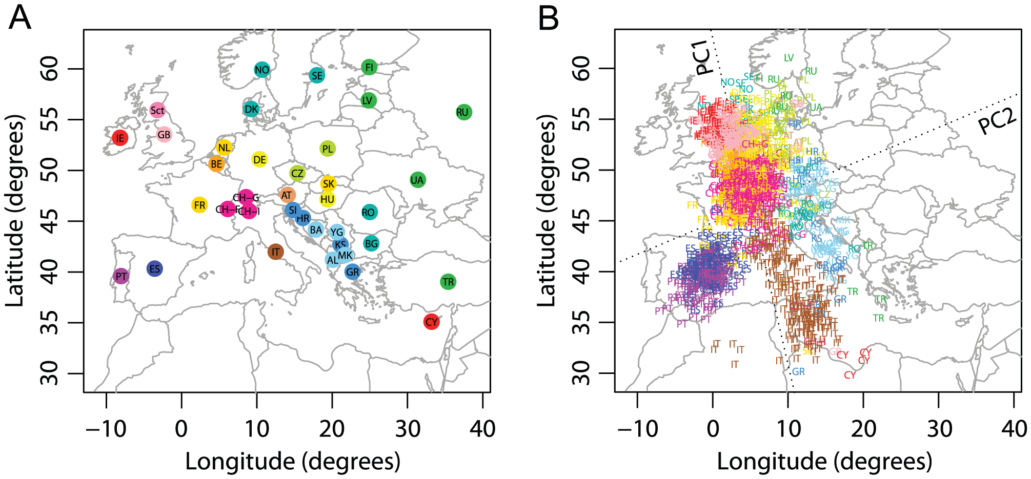
Figure 3, from: Wang C, Zöllner S, Rosenberg NA (2012) A Quantitative Comparison of the Similarity between Genes and Geography in Worldwide Human Populations. PLOS Genetics 8(8): e1002886. https://doi.org/10.1371/journal.pgen.1002886
Expectations in specific genetic conditions
For conditions like cystic fibrosis (deficiency in cystic fibrosis transmembrane conductance regulator, CFTR), where the most common known causes of disease are due to a variant that is inherited rather than spontaneous, PCA is expected reveal clustering within certain population groups, attributed to shared ancestral lineages. By default, cases with a shared variant are likely to cluster together in population groups because their DNA recombinations will have shared lineages (including the variant of interest AND all of the other blocks of the genome). Otherwise, they would not have inherited the block of DNA containing this variant. This is opposed to spontaneous variants, which appear independently of ancestral haplotypes and are unrelated to the distribution patterns PCA might reveal.
Comparison with viral genetics
Human genetics is generally more complex than viral genomes which depend on asexual reproduction. However, parallels can be drawn with viral genetics, where tracking variants is often more straightforward due to less genetic diversity compared to humans.
This screenshot from Nextstrain Viral Epidemiology shows the clade of viruses across their genetic tree and physical location. In this case, the complication of recombination is removed and we simply have direct clonal descent and some spontaneous variants occuring.
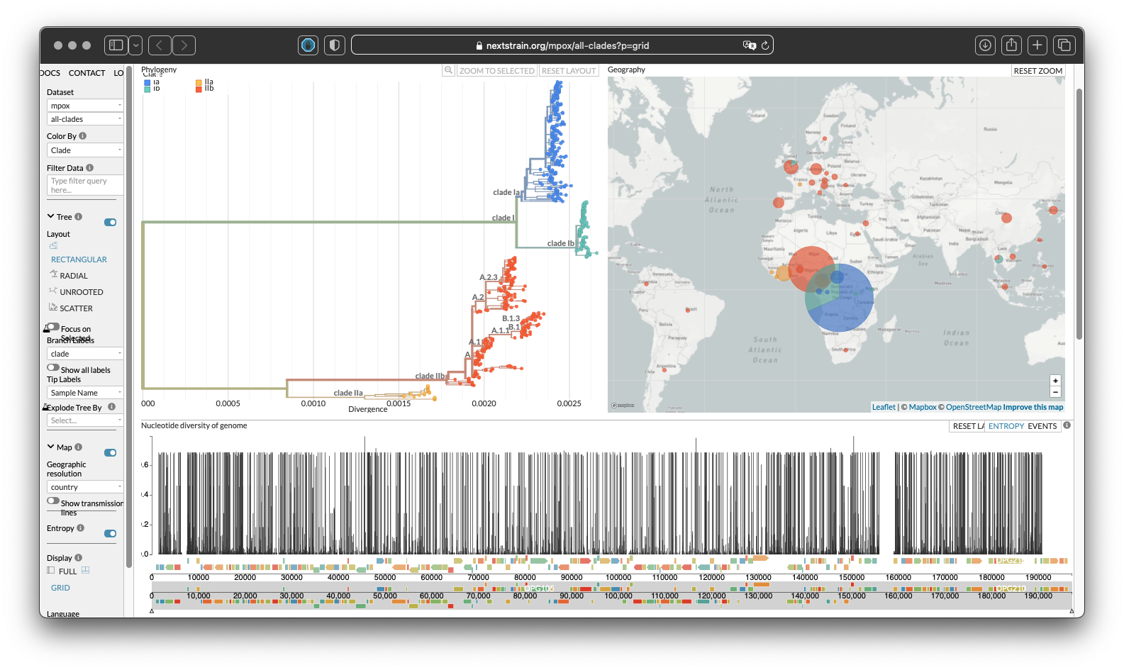
Figure 4: Screenshot of Nexstrain - Genomic epidemiology of mpox viruses across clades Data updated 2025-01-04. Enabled by data from GenBank. Showing 549 of 549 genomes.
Analysis for unknown variants
Generally, association testing is focused on finding some shared genetic feature among affected patients. PCA is used to remove the background noise of benign haplotype blocks which are shared by inheritance. Some unique patterns belong to different population groups which would otherwise appear as if they are related to disease. After correcting for population structure with PCA, we hope to ignore those false positives and only identify variants that are truly associated (i.e. potentially causal) with disease. Our intention is that this association will subsequently give was to causal inference with additional analysis.
Sibling and related samples
The strategy for keeping a single sibling, or other approaches, should be carefully assessed for an analysis.
Closely related individuals, such as siblings will be seen to cluster closely together due to their very closely shared ancestry. Any haplotype block that one sibling carries, is likely to be present for the second sibling also. In a statistical analysis, if they method relies on detecting enriched features, such as the haplotype block in the case of GWAS, then the signal will be fasly amplified since it doubled, by default, for siblings. Typically in GWAS and other similar analysis it is important to count only one sibiling from a family in the analysis cohort. KING software (Kinship-based INference for Gwas) is often used for estimating kinship coefficients and inferring IBD segments for all pairwise relationships. This can also use the same input Plink format data as the PCA steps with Plink. https://www.kingrelatedness.com/manual.shtml
The following explanation example from KING is pertinent - even if it is not required for an analysis - which we quote here:
KINSHIP INFERENCE –kinship estimates pair-wise kinship coefficients using the KING-Robust algorithm described in the original KING paper. If pedigrees are documented in the .fam file (see LINKAGE format examples), kinship coefficients can be estimated within families. Note if each FID is unique and no pedigrees are provided, then the within-family inference will be skipped. The output for within-family relationship checking using –kinship (saved in file king.kin) will look like this:
FID     ID1     ID2     N_SNP   Z0      Phi     HetHet  IBS0    Kinship Error
28      1       2       2359853 0.000   0.2500  0.162   0.0008  0.2459  0
28      1       3       2351257 0.000   0.2500  0.161   0.0008  0.2466  0
28      2       3       2368538 1.000   0.0000  0.120   0.0634  -0.0108 0
117     1       2       2354279 0.000   0.2500  0.163   0.0006  0.2477  0
117     1       3       2358957 0.000   0.2500  0.164   0.0006  0.2490  0
117     2       3       2348875 1.000   0.0000  0.122   0.0616  -0.0017 0
1344    1       12      2372286 0.000   0.2500  0.149   0.0003  0.2480  0
1344    1       13      2370435 0.000   0.2500  0.148   0.0003  0.2465  0
1344    12      13      2374888 1.000   0.0000  0.117   0.0582  0.0003  0
Each row above provides information for one pair of individuals. The columns are
FID: Family ID for the pair
ID1: Individual ID for the first individual of the pair
ID2: Individual ID for the second individual of the pair
N_SNP: The number of SNPs that do not have missing genotypes in either of the individual
Z0: Pr(IBD=0) as specified by the provided pedigree data
Phi: Kinship coefficient as specified by the provided pedigree data
HetHet: Proportion of SNPs with double heterozygotes (e.g., AG and AG)
IBS0: Porportion of SNPs with zero IBS (identical-by-state) (e.g., AA and GG)
Kinship: Estimated kinship coefficient from the SNP data
Error: Flag indicating differences between the estimated and specified kinship coefficients (1 for error, 0.5 for warning)
The default kinship coefficient estimation only involves the use of SNP data from this pair of individuals, and the inference is robust to population structure. A negative kinship coefficient estimation indicates an unrelated relationship. The reason that a negative kinship coefficient is not set to zero is a very negative value may indicate the population structure between the two individuals. Close relatives can be inferred fairly reliably based on the estimated kinship coefficients as shown in the following simple algorithm: an estimated kinship coefficient range >0.354, [0.177, 0.354], [0.0884, 0.177] and [0.0442, 0.0884] corresponds to duplicate/MZ twin, 1st-degree, 2nd-degree, and 3rd-degree relationships respectively. Relationship inference for more distant relationships is more challenging. A plot of the estimated kinship coefficient against the proportion of zero IBS-sharing is highly recommended. In the absence of population structure, relationship inference can also be carried out using an alternative algorithm through parameter “–homog”.
Manichaikul A, Mychaleckyj JC, Rich SS, Daly K, Sale M, Chen WM (2010) Robust relationship inference in genome-wide association studies. Bioinformatics 26(22):2867-2873 Abstract PDF Citations.
Population structure in other omics
In GWAS, PCA is employed to control for population structure by including the top principal components in the analysis. The applicability of this method extends to other omics analsis, including RNAseq differential expression (DE), which quantitatively test for RNAseq abundance, protein abundance, or multi-omic data (mixed DNA, RNA, and protein), especially when the analysis resembles a simple association test similar to Plink’s –assoc. It is both necessary and effective to use PCA in RNAseq DE, for example, to manage population structure. Analogous to its use in GWAS, where PCA corrects for population structure in genetic data, RNAseq-based genetic principal components (RG-PCs) can be computed and employed as covariates in DE analyses. This strategy reduces confounding effects due to population stratification, thereby improving the accuracy and reliability of the results. For more reading see:
- Fachrul et al. (2023). Direct inference and control of genetic population structure from RNA sequencing data. https://www.nature.com/articles/s42003-023-05171-9
- Storey, J. D. et al. Gene-expression variation within and among human populations. Am. J. Hum. Genet. 80, 502–509 (2007). https://doi.org/10.1086%2F512017
- Thami, P. K. & Chimusa, E. R. Population structure and implications on the genetic architecture of HIV-1 phenotypes within Southern Africa. Front. Genet. 10, 905 (2019).https://doi.org/10.3389%2Ffgene.2019.00905
- Li, J., Liu, Y., Kim, T., Min, R. & Zhang, Z. Gene expression variability within and between human populations and implications toward disease susceptibility. PLoS Comput. Biol. 6, e1000910 (2010).https://doi.org/10.1371%2Fjournal.pcbi.1000910
- Jovov, B. et al. Differential gene expression between African American and European American colorectal cancer patients. PLoS ONE 7, e30168 (2012).https://doi.org/10.1371%2Fjournal.pone.0030168
- Price, A. L. et al. Principal components analysis corrects for stratification in genome-wide association studies. Nat. Genet. 38, 904–909 (2006).https://doi.org/10.1038%2Fng1847
Lastly, the abstract from the following says why the the answer is not always commonly reported:
- Shiquan Sun, Michelle Hood, Laura Scott, Qinke Peng, Sayan Mukherjee, Jenny Tung, Xiang Zhou, Differential expression analysis for RNAseq using Poisson mixed models, Nucleic Acids Research, Volume 45, Issue 11, 20 June 2017, Page e106, https://doi.org/10.1093/nar/gkx204
Identifying differentially expressed (DE) genes from RNA sequencing (RNAseq) studies is among the most common analyses in genomics. However, RNAseq DE analysis presents several statistical and computational challenges, including over-dispersed read counts and, in some settings, sample non-independence. Previous count-based methods rely on simple hierarchical Poisson models (e.g. negative binomial) to model independent over-dispersion, but do not account for sample non-independence due to relatedness, population structure and/or hidden confounders.