Finite Markov Decision Process (MDP)

Last update: 20250322

In reinforcement learning, the agent interacts with an environment through a well-defined interface. The agent’s goal is to maximise cumulative rewards by selecting actions that influence the state of the environment. Key concepts include:

• Goals: The objectives the agent strives to achieve.
• Rewards: Immediate feedback received after performing an action.
• Returns: The total accumulated reward over an episode.
• Episodes: Sequences of states, actions, and rewards that conclude when a terminal condition (goal achieved or failure) is met.

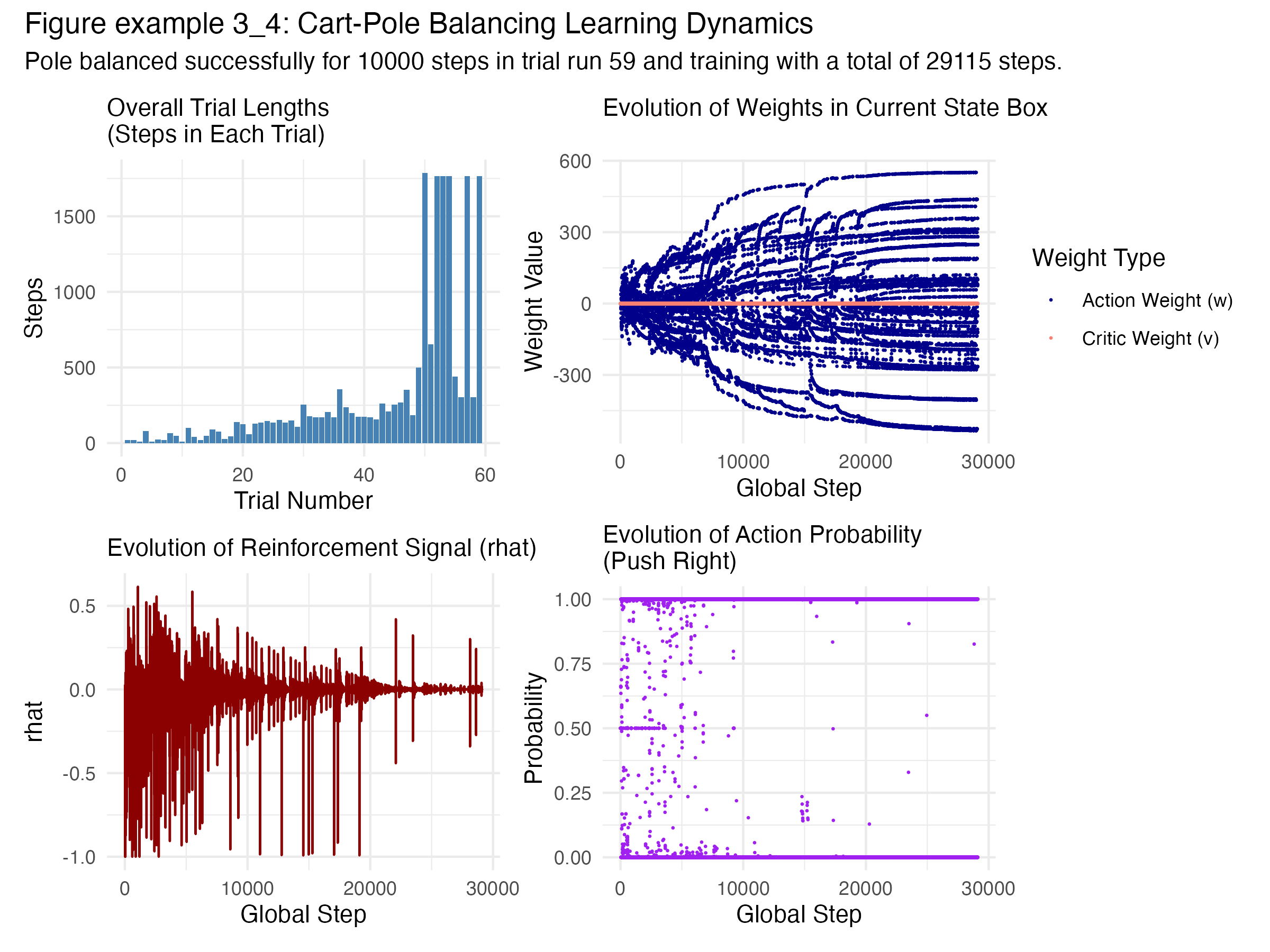
These ideas are exemplified in the cart pole balancing problem, where the agent must keep a pole balanced on a moving cart. Here, the environment continuously provides rewards based on the pole’s stability, and an episode ends when the pole falls or the cart leaves a designated area.

Moving on to a discrete setting, the gridworld example represents a simple Markov Decision Process (MDP) with a 5×5 grid where each cell is a state. The environment is defined by standard grid dynamics, with a discount factor (γ = 0.9) and a termination criterion based on a small change threshold (1e–6). The agent can move in one of four directions (up, right, down, left), but there are two special states (A and B) that trigger exceptional transitions:

• Special Transitions:
  • When in state A (cell at (1,4)), any action leads the agent to state A’ (cell at (1,0)) with a reward of +10.
  • When in state B (cell at (3,4)), any action leads the agent to state B’ (cell at (3,2)) with a reward of +5.

For other states, moving off the grid results in staying in the same state with a penalty of –1, while valid moves provide zero immediate reward.

Two main value functions are computed:

• Uniform Policy Value Function (V):
  This is computed by averaging the backups (expected returns) over all actions, simulating a uniform random policy.
• Optimal Value Function (V*):
  Here, the Bellman optimality equation is used (taking the maximum over actions) to iteratively compute the optimal state-value function. Alongside V*, the optimal policy (π*) is derived, indicating for each state the action(s) that maximise the expected return.

The resulting figures illustrate these concepts:

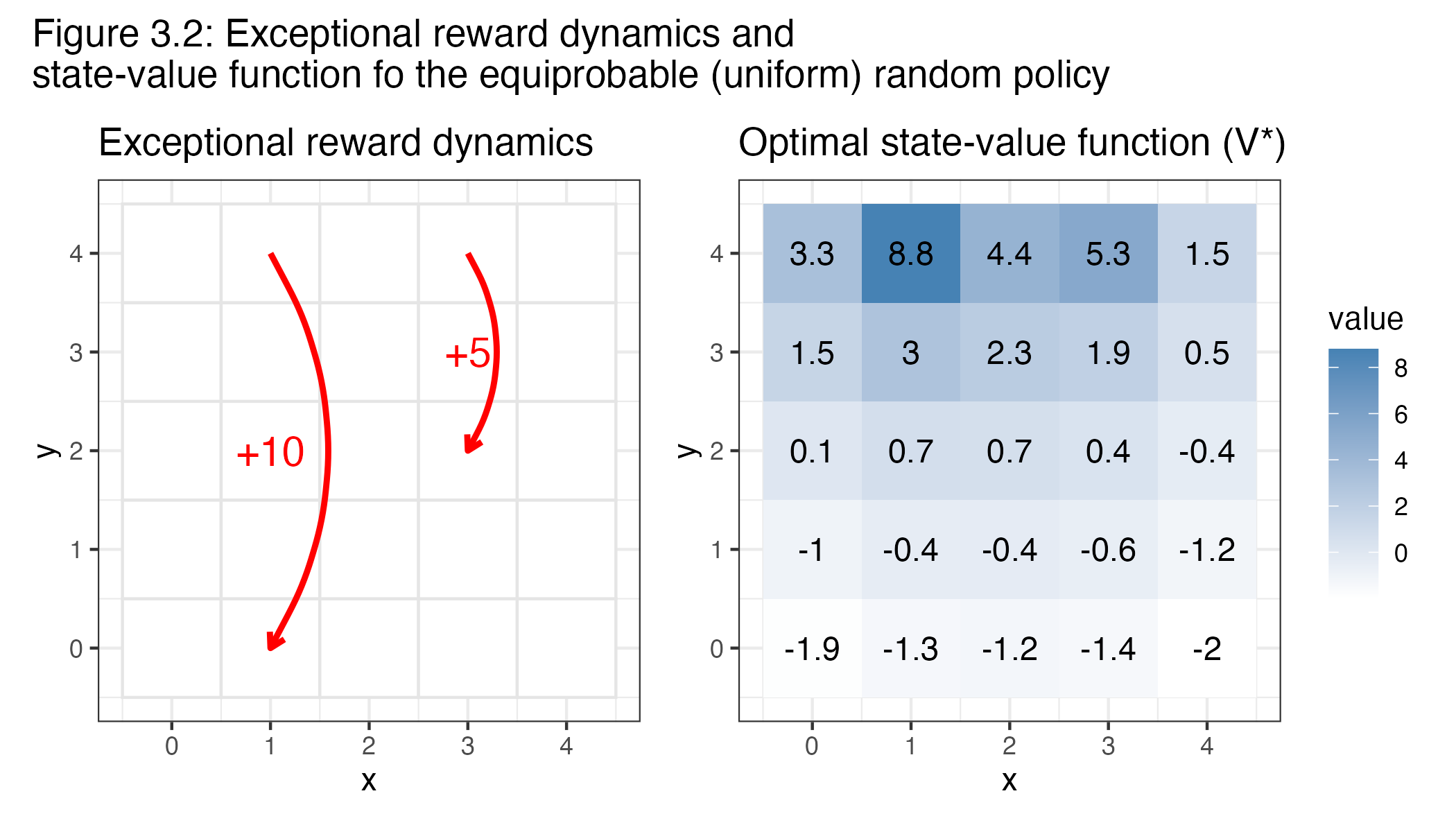
• Figure 3.2 (Combined Uniform Policy and Exceptional Dynamics):
  • Left Panel – Exceptional Reward Dynamics:
    This plot shows the grid with curved red arrows that indicate the special transitions from state A to A’ and from state B to B’. The arrows are annotated with the respective rewards (+10 and +5), highlighting the exceptional dynamics of the MDP.
  • Right Panel – Uniform State-Value Function:
    Here, the state-value function computed under a uniform random policy is visualised. Each cell displays its value (printed as text) and is colour-coded, providing a clear picture of how the environment’s dynamics (including the special transitions) propagate values throughout the grid.

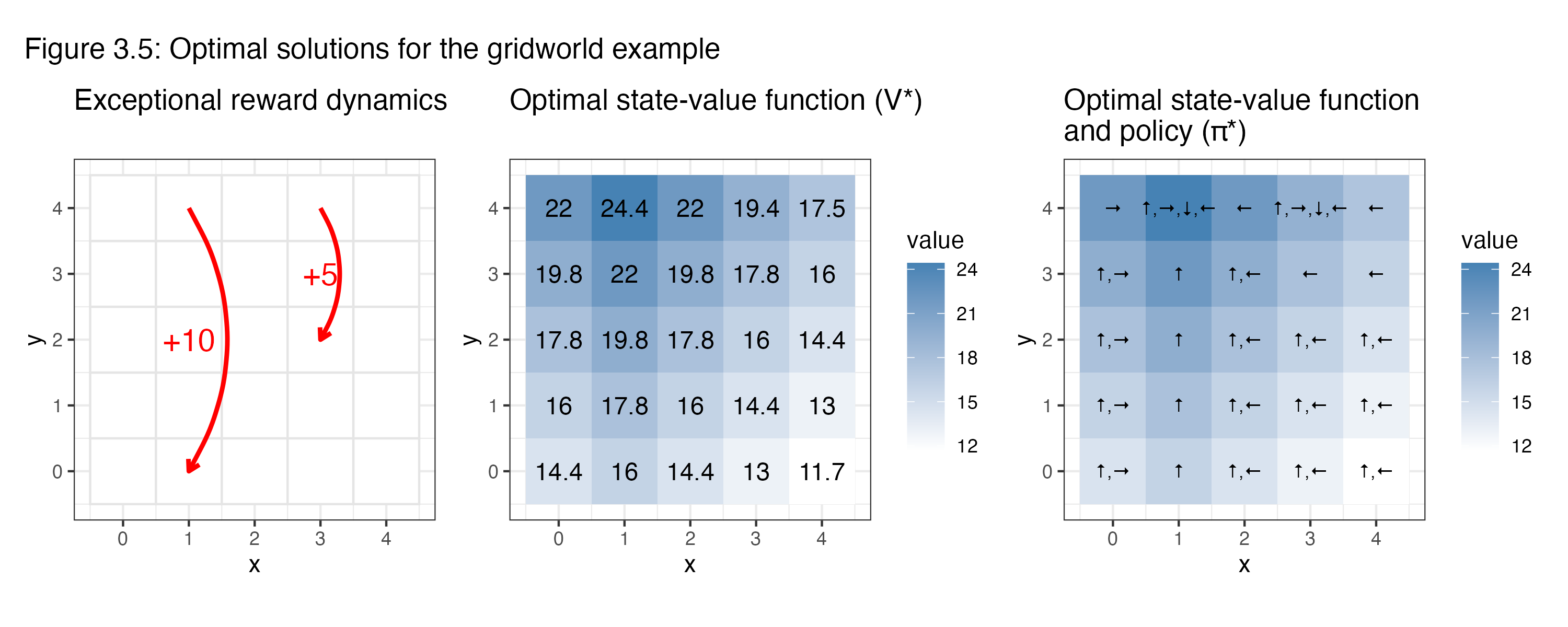
• Figure 3.5 (Combined Optimal Value and Policy):
  This composite figure consists of three subplots:
  1. Exceptional Reward Dynamics: (Same as in Figure 3.2)
     Reiterates the exceptional transitions to contextualise the optimal calculations.
  2. Optimal State-Value Function (V*):
     The computed optimal values are displayed in each cell with both numerical annotations and a colour gradient, illustrating the effect of choosing the best possible actions.
  3. Optimal Policy (π*):
     This plot overlays directional arrows inside each grid cell, representing the optimal action(s) derived from V*. The arrows correspond to the directions (up, right, down, left) that yield the highest expected return. In some cells, multiple arrows appear if several actions are equally optimal.

Together, these figures provide a comprehensive visualisation of the theory behind reinforcement learning, illustrating both the agent–environment interface (as demonstrated in the pole balancing task) and the formal MDP framework (as implemented in the gridworld example). They demonstrate how rewards and returns are generated in episodes, how value functions are computed, and how optimal decision-making is represented both in value terms and as explicit action choices within the grid.