Last update: 20241217
Design QV SNV INDEL v1
Qualifying variant protocol for SNV INDEL v1
Protocol name: design_qv_snvindel_v1
Introduction
This pages summarises the qualifying variant (QV) settings used for QV SNV INDEL v1. QV defines those variants which remain after filtering for use in downstream analysis. In general, most choices are based on well established best practices. For any subjective choices of thesholds, we will rely on evidence-based reasoning. However, it is important for users to understand whether their QV is suited to a particular context. For example, a GWAS analysis typically relies on the presence of common shared variants while a clinical genetics report might focus on rare novel variants. Conversely, cohort-level a genetic relationship matrix for use in statistical analysis might rely on some but not all of the QV steps (such as dropping some filters so that haplotypes can be correcly represented). You can read about QV in this review 1 https://www.nature.com/articles/s41576-019-0177-4/.
Examples of QV sets are: (1) QC-only QV resulting in a very large remaining variant dataset, e.g. >500’000 variants per subject. (2) Rare disease QV resulting in a small dataset with strict filters, e.g. 10’000 variants per subject. (3) Flexible QV resulting in disease-causing candidate variants with modest filtering to balance QC and false positives, e.g. <100’000 variants per subject.
Several QV protocols can be piped together to create increasingly filtered datasets to match the needs at a certain stage of analysis. It is also typical that different analysis from QVs sets are used and the final results from each step are merged to cover multiple scenarios. For example, SNV/INDEL QV + CNV QV + rare disease known QV + statitcal assossiation QC may be merged to reach the final combined analysis of (1) single case-level known disease causing results with (2) newly identified cohort-level genes associated with disease.
The following figure 1 from Hillman et. al. 2 is a typical illustration of QV workflow. We do not use this reference for any analysis. The figure is simply shown for illustration. Figure 2 from Povysil et al. 1 provides an example of the application of QV in an analysis.
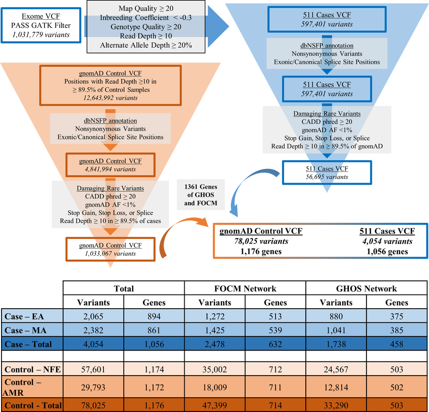 Figure 1: From Hillman et. al. 2. Variant filtering and annotation workflow with summative case and control variant and gene counts. Top. General workflow and filtering parameters applied to data. Bottom. Table summarizing total qualifying variant and gene counts by ethnicity and in total for cases and controls. Variant counts represent the number of unique qualifying variant loci identified in each ethnicity and network. Gene counts represent the number of genes containing at least one qualifying variant in each network and ethnicity. AMR, American Latino; CADD, combined annotation dependent depletion; dbNSFP, database of non-synonymous single-nucleotide variant functional predictions; EA, European Americans; FOCM, Folate and One-Carbon Metabolism; GATK, Genome Analysis Toolkit; GHOS, Glucose Homeostasis and Oxidative Stress; gnomAD, genome aggregation database; MA, Mexican Americans; NFE, Non-Finnish Europeans; VCF, variant call format.
Variables and thresholds
This protocol shown here (SNV INDEL v1) is considered as the flexible format.
QC-only QV
- [QC]
01_fastp.shThe tool fastp is used for QC. FASTQ that fail are investigated or removed. See fastp for more. - [QC]
03b_collectwgsmetrics.shBAMs that fail are investigated or removed. See metrics_CollectWgsMetrics for more. - [QC]
05_rmdup_merge.shis used to mark optical duplicates. See GATK Duplicates for more. - [QC]
07_haplotype_caller.shused-ERC GVCFmode. This does not remove variants but unlikeBP_RESOLUTION,GVCFmode condenses non-variant blocks which could be misunderstood later as missing if not recongnised by the user, for example in a genotype matrix which has been merged with other cohorts. See VCF and VCF and gVCF for more. - [QC]
07c_qc_summary_stats.shis used to log QC. This implementsbcftools stats(https://samtools.github.io/bcftools/bcftools.html#stats) and subsequently the bcftoolsplot-vcfstats(https://samtools.github.io/bcftools/bcftools.html#plot-vcfstats) usingpython -m venv envQCplotwith matplotlib. Subjects fail are investigated or removed. See metrics_bcftoolsstats. - [QC] !Not used Large cohort hard-filter. The following step is generllay useful before VQSR (shown later), however since our cohort is likely to contain some large populations of unrelated patients with the same causal genetic variants, we skip it to avoid loosing them. (https://gatk.broadinstitute.org/hc/en-us/articles/360035531112--How-to-Filter-variants-either-with-VQSR-or-by-hard-filtering) [A] Hard-filtter a large cohort callset on ExcessHet (https://gatk.broadinstitute.org/hc/en-us/articles/360036726851-ExcessHet) using VariantFiltration (https://gatk.broadinstitute.org/hc/en-us/articles/360036350452-VariantFiltration). ExcessHet filtering applies only to callsets with a large number of samples, e.g. hundreds of unrelated samples. Small cohorts should not trigger ExcessHet filtering as values should remain small. Note cohorts of consanguinous samples will inflate ExcessHet, and it is possible to limit the annotation to founders for such cohorts by providing a pedigree file during variant calling. For example,
"ExcessHet > 54.69"produces a VCF callset where any record with ExcessHet greater than 54.69 is filtered with the ExcessHet label in the FILTER column. The phred-scaled 54.69 corresponds to a z-score of -4.5. If a record lacks the ExcessHet annotation, it will pass filters. If run, this step would be followed byMakeSitesOnlyVcf(https://gatk.broadinstitute.org/hc/en-us/articles/360036346712-MakeSitesOnlyVcf-Picard-) to speed up analysis. - [QC]
10_vqsr.shapplies the Variant Quality Score Recalibration (VQSR) method in GATK, a sophisticated approach used to assess variant quality and filter out sequencing and data processing artifacts. Our settings are shown in table below; they include priors for SNPs fromHapMap=15.0,Omni=12.0,1000G=10.0, andTruth Sensitivity = 99.7, for INDELSMills 1KG=12.0,dbSNP=2.0andTruth Sensitivity=95and across all, the annotations QD, MQRankSum, ReadPosRankSum, FS, SOR. This two-step procedure begins with building a recalibration model that evaluates the relationship between variant annotations, such as Quality by Depth (QD), Mapping Quality (MQ), and Read Position Rank Sum Test (ReadPosRankSum), against the likelihood that a variant is genuine. Key resources like HapMap and Omni 2.5M SNP chip array data are leveraged to train this model adaptively. By employing an adaptive error model and a Gaussian mixture model, VQSR provides a score known as VQSLOD (Variant Quality Score Log Odds), which indicates the likelihood of each variant being true. The VQSLOD scores are incorporated into the variant call file (VCF), allowing for highly precise and flexible filtering. The overall aim of VQSR is to allocate a calibrated probability to each variant, surpassing traditional methods that rely strictly on fixed annotation value thresholds. This technique is especially crucial in contexts where accuracy in variant filtering significantly impacts subsequent analyses and conclusions, particularly in medical genomics research. Population resource files are publically available at https://console.cloud.google.com/storage/browser/broad-references/hg38/v0/. Further reading about techniques here https://gatk.broadinstitute.org/hc/en-us/articles/360035531112--How-to-Filter-variants-either-with-VQSR-or-by-hard-filtering and here https://gatk.broadinstitute.org/hc/en-us/articles/360035531612-Variant-Quality-Score-Recalibration-VQSR?id=1259. - [QC] see
10b_qc_summary_statsfor plink logs${QC_SUMMARY_STATS}/vqsr/${QV_MODEL}_chr${INDEX}_summary_stat.log - [QC] Optional CollectVariantCallingMetrics. An example is shown here https://gatk.broadinstitute.org/hc/en-us/articles/360035531112--How-to-Filter-variants-either-with-VQSR-or-by-hard-filtering and documentation here https://gatk.broadinstitute.org/hc/en-us/articles/360036363592-CollectVariantCallingMetrics-Picard.
- [QC] Optional Other Picard metrics which are not in use: https://broadinstitute.github.io/picard/picard-metric-definitions.html.
- [QC]
11_genotype_refinement.shGenotype Refinement workflow is a collection of steps https://gatk.broadinstitute.org/hc/en-us/articles/360035531432-Genotype-Refinement-workflow-for-germline-short-variants. We will continue to add steps to our current implementation. For example, when we have trio studies we can provide more nuanced variant confidence methods. We currently use (1)CalculateGenotypePosteriors: This tool refines genotype probabilities using family data or population allele frequencies. We use gnomADaf-only-gnomad.hg38.vcf.gz. It enhances the initial genotype likelihoods from variant callers, ensuring accuracy especially when incorporating trio and population data. This step reduces false positives and improves genotype precision. https://gatk.broadinstitute.org/hc/en-us/articles/360037226592-CalculateGenotypePosteriors. (2)VariantFiltration: This stage applies filters. We useGQ < 20on genotype quality scores to flag lower confidence genotypes. It refines variant call quality by annotating individual genotypes based on specified criteria, helping to isolate high-confidence calls from potential errors. https://gatk.broadinstitute.org/hc/en-us/articles/360041850471-VariantFiltration. - [QC] The same stats as
10b_qc_summary_statsfor plink logs are run in step11_genotype_refinement.sh. - [Filter]
12_pre_annotation_processing.sh. We apply the followingbcftools filterwith (1) QUAL>=30: Filters for variants where the quality score is 30 or higher. The quality score (QUAL) represents the confidence in the correctness of the variant call. (2) INFO/DP>=20: Filters for variants where the total depth of quality base calls (DP in the INFO field of a VCF file) is 20 or more. This is a measure of the total amount of sequencing data that supports the variants in the file. (3) FORMAT/DP>=10: Applies a filter to each individual sample in the VCF file, ensuring that the depth of reads for each genotype call is 10 or more. This ensures that each genotype call in every sample has sufficient data supporting it. (4) FORMAT/GQ>=20: Ensures that the genotype quality (GQ) for each sample’s call is 20 or above. The genotype quality score expresses the confidence in the assignment of the genotype at that specific locus. (5) Then GATKSelectVariantsis subsequently applied with--exclude-filtered,--exclude-non-variants, and--remove-unused-alternates. - [QC]
12_pre_annotation_processing.shalso contains the steps using vt (variant tool) https://genome.sph.umich.edu/wiki/Vt to run (1)variant decomposehttps://genome.sph.umich.edu/wiki/Vt#Decompose a complex operation to ensure that multiallelic variants (a feature of VCF format) are split into distinct observations to remove errors in downstream analysis and (2)variant normalisationhttps://genome.sph.umich.edu/wiki/Variant_Normalization a proof-bacjed procedure to ensure that variant representations conform to a consensus format. See Tan et. al 3. A variant is parsimonious if and only if it is represented in as few nucleotides as possible without an allele of length 0. Futher reading here https://genome.sph.umich.edu/wiki/Vt#Normalization - [Filter] 13_pre_annotation_MAF.sh runs data preparation steps including a filter with
vcftools--max-mafusing the source variableMAF_value="0.4". This step is simply for reducing the data size to remove highly common variants. We do not expect more than 40% of the cohort to share a relavent variant.
Rare disease QV (run after QC-only QV)
- ACMG filtering ACMG criteria and scoring
- Variant interpretation in disease. This final step is used in a case-by-case basis to assess whether automated analysis agrees with the consensus clinical genetics approach.
Table 1. VQSR settings
| VQSR Settings | Explanation |
|---|---|
| SNP Mode | |
| - HapMap: known=false, training=true, truth=true, prior=15.0 | Used as a high-confidence reference set for training the recalibration model. |
| - Omni: known=false, training=true, truth=false, prior=12.0 | Provides additional training data derived from Omni genotyping arrays. |
| - 1000G: known=false, training=true, truth=false, prior=10.0 | Utilizes data from the 1000 Genomes Project to inform the model on common SNP variations. |
| - Annotations: QD, MQ, MQRankSum, ReadPosRankSum, FS, SOR | Annotations are metrics used to predict the likelihood of a variant being a true genetic variation versus a sequencing artifact. They include quality by depth, mapping quality, mapping quality rank sum test, read position rank sum test, Fisher’s exact test for strand bias, and symmetric odds ratio of strand bias. |
| - Truth Sensitivity Filter Level: 99.7 | Specifies the percentage of true variants to retain at a given VQSLOD score threshold, set here to capture 99.7% of true variants. |
| INDEL Mode | |
| - Mills: known=false, training=true, truth=true, prior=12.0 | Utilizes the Mills and 1000G gold standard indel dataset for high-accuracy recalibration of indels. |
| - dbSNP: known=true, training=false, truth=false, prior=2.0 | Includes known indel sites from the dbSNP database to enhance the detection and filtering process. |
| - Annotations: QD, MQRankSum, ReadPosRankSum, FS, SOR | Same as for SNPs, these annotations are critical for assessing the likelihood of indels being true genetic variations rather than errors. |
| - Truth Sensitivity Filter Level: 95 | This setting defines the percentage of true indels to retain, aiming to capture 95% of true indels at the specified VQSLOD threshold. |
Variables file
During analysis we source the following variables.sh file. We will continue to update this so that all QV variables and thresholds are included here. In future releases, we plan to have each version of the variables file indentified with sensible names like variables_dna_snvindel_v1 etc.
# This script is meant to be sourced, not executed. To use the variables
# defined in this script, use the command `source variables.sh` in your
# own scripts.

# main paths
HOME="/project/home/lawless"
DATA="${HOME}/data/wgs"
PROD="/project/data/prod"

# processed data
STUDYBOOK_DIR="${DATA}/study_book_data"
FASTP_DIR="${DATA}/fastp"
FASTP_METRICS_DIR="${DATA}/fastp_reports"
BAM_DIR="${DATA}/bam"
SAMSORT_DIR="${DATA}/samsort"
RMDUP_DIR="${DATA}/rmdup"
RMDUP_MERGE_DIR="${DATA}/rmdup_merge"
BQSR_DIR="${DATA}/bqsr"
BQSR_DIR_HOLD="${DATA}/bqsr_hold"
KNOWN_SITES="${HOME}/data/db/known_sites"
HC_DIR="${DATA}/hc"
HC_RENAMED_DIR="${DATA}/hc_renamed"
GENOMICS_DB_IMPORT_DIR="${DATA}/genomics_db_import"
GENOTYPE_GVCF_DIR="${DATA}/genotype_gvcf"
VQSR_DIR="${DATA}/vqsr"
GENOTYPE_REFINEMENT_DIR="${DATA}/genotype_refine"
PRE_ANNOTATION_DIR="${DATA}/pre_annotation"
PRE_ANNOTATION_MAF_DIR="${DATA}/pre_annotation_maf"
ANNOTATION_DIR="${DATA}/annotation"
ANNOTATION_GNOMAD_DIR="${DATA}/annotation_gnomad"
POSTANNOSPLIT="${DATA}/annotation_split"
POSTVCF2TABLE="${DATA}/vcf2table"
VIRTUAL_PANEL_DIR="${DATA}/virtual_panel"
VCFLIB_DIR="${DATA}/vcflib_out"
VARLEVEL_DIR="${DATA}/variant_level"
VAL_DIR="${DATA}/validation"
MAF_value="0.4"
GNOMAD_value="0.002"
DATABASE_DIR="${HOME}/data/db"
dbNSFP_grch38="${DATABASE_DIR}/dbnsfp/dbNSFP4.4a_grch38_v3.gz"
THOUSAND_GENOMES="/project/home/lawless/data/ref/1000genomes/"
PCA_BIPLOT_1KG="${DATA}/pca_biplot_1kg"
SMOOVE="${DATA}/smoove"
VSAT="${DATA}/plink_skat_vsat"
QC_SUMMARY_STATS="${DATA}/qc_summary_stats"

# src
PROJECT="${HOME}/wgs"
SRC="${PROJECT}/src"

# ref
REF="/project/home/lawless/data/ref/bgzip_fasta/GCA_000001405.15_GRCh38_no_alt_analysis_set.fna.gz"
REF_NONZIP="/project/home/lawless/data/ref/bgzip_fasta/GCA_000001405.15_GRCh38_no_alt_analysis_set.fna"
REF_SHARED="/project/data/shared/processed_data/GCA_000001405.15_GRCh38_no_alt_analysis_set.fna"
SV_EXCLUDE_BED="/project/home/lawless/data/ref/bed_annotaions/exclude.cnvnator_100bp.GRCh38.20170403.bed"
VEP_VERSION="95"
VEP_CACHE_DIR="${DATABASE_DIR}/vep${VEP_VERSION}/cache"
VEP_PLUGIN_DIR="${DATABASE_DIR}/vep${VEP_VERSION}/plugins"
The use of QV in analysis plan
QV are a logical necessity of data cleaning and preperation. Labelling then the single umbrella of QV is useful for simplicity. In reality the steps of QV can be sepated and result from a mixture of different steps or sources. Figure 2 from Povysil et al. 1 provides an example of the application of QV in an analysis.
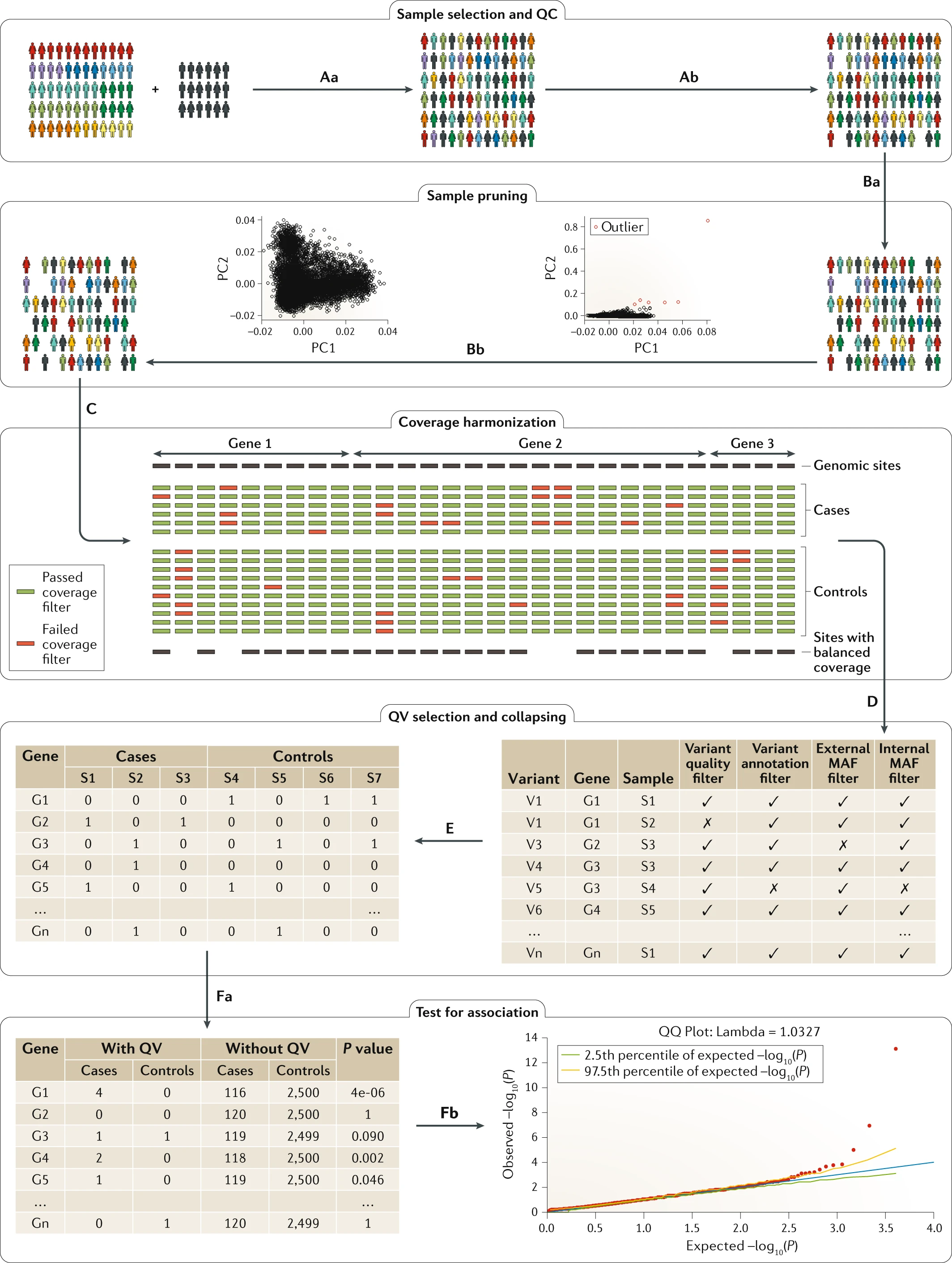
Figure 2. From Povysil et. al 1: Outline of the standard collapsing analysis approach. First, cases and matching controls are selected (part Aa), and the same sample-level quality control (QC) is performed for cases and controls (part Ab). The sample-pruning level comprises relatedness pruning (part Ba) and the removal of population outliers based on principal components (PCs) (part Bb). All the remaining samples are used to perform coverage harmonization (part C), in which sites and therefore variants that show coverage differences between cases and controls are pruned. All remaining variants are used for qualifying variant (QV) selection (part D), in which various filters, including internal and external minor allele frequency (MAF) filters, are applied. The selected QVs are used to build the gene-by-individual collapsing matrix (part E), which indicates the presence of at least one QV. Finally, each gene is tested for an association between QV status and the phenotype of interest (part Fa), and the results can be evaluated by means of a quantile–quantile (QQ) plot (part Fb).
References
Povysil, G. et al., 2019. Rare-variant collapsing analyses for complex traits: guidelines and applications. Nature Reviews Genetics, 20(12), pp.747-759. DOI: 10.1038/s41576-019-0177-4. ↩ ↩2 ↩3 ↩4
Hillman, P., Baker, C., Hebert, L., Brown, M., Hixson, J., Ashley-Koch, A., Morrison, A.C., Northrup, H. and Au, K.S. (2020), Identification of novel candidate risk genes for myelomeningocele within the glucose homeostasis/oxidative stress and folate/one-carbon metabolism networks. Mol Genet Genomic Med, 8: e1495. https://doi.org/10.1002/mgg3.1495 ↩ ↩2
Adrian Tan, Gonçalo R. Abecasis, Hyun Min Kang, Unified representation of genetic variants, Bioinformatics, Volume 31, Issue 13, July 2015, Pages 2202–2204, https://doi.org/10.1093/bioinformatics/btv112 ↩