GWAS analysis
Last update: 20240929
Table of contents
Overview
Genome-Wide Association Studies (GWAS) are research approaches used to associate specific genetic variations with particular diseases. By analysing genetic variants across multiple samples, GWAS aim to identify genetic markers linked to disease traits. This process involves several stages, from data preparation to statistical analysis and visual representation of results.
Data Preparation
VCF to PLINK Conversion (plink_1_vcf_to_plink.sh)
This initial script converts joint genotyped cohort VCF files, which are split per chromosome, into a more manageable format using PLINK. The VCF files are decompressed, and the data is converted into binary format (BED, BIM, FAM files), which is suitable for fast processing in subsequent analysis steps.
Covariate and Phenotype Preparation (plink_2_covar.sh)
This script prepares phenotype information and covariates, which are crucial for adjusting the GWAS analysis to prevent confounding results. It involves generating phenotype files from structured data sources and integrating them with genetic data files (FAM files). Additionally, Principal Component Analysis (PCA) is run on the genotype data to correct for population stratification, which is a critical step to ensure that genetic associations are not due to population structure differences.
PCA: The population structure of genetic data can be controlled in GWAS by applying PCA. To simulate synthetic data or to understand the poplutation in cohort data we could compare it to population of classified ancestries such as the 1000 genomes project. In our exploration stages we produce the PCA bi-plot for 1000 Genomes Phase III - Version 2 (https://www.biostars.org/p/335605/) merged with our study data.
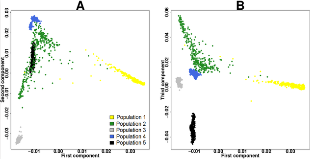 Figure 1. PCA from 1000 genomes project data by Kevin Blighe via biostars.org.
Statistical Analysis
Association Testing (plink_3_assoc.sh)
Once data preparation is complete, this step involves cleaning the data further, including filtering by genotype frequency. The association testing is then carried out using PLINK, which tests for correlations between each genetic variant and the trait of interest while adjusting for covariates and significant principal components from the PCA. The results are consolidated into association files (.assoc) for each chromosome.
Visualisation of Results
Plotting Results (plink_4_plot.sh and plink_4_plot.R)
The final step involves visualising the results of the GWAS. The plink_4_plot.sh script calls an R script to generate a Manhattan plot and a QQ plot. These plots are essential for interpreting GWAS results:
- Manhattan Plot: This plot visualises the -log10(p-values) of the association tests across all chromosomes, highlighting genomic regions that surpass the genome-wide significance threshold.
- QQ Plot: This plot helps assess whether the p-values conform to the expected distribution under the null hypothesis of no association, which helps in identifying potential issues like population stratification, cryptic relatedness, or differential genotyping quality.
The output from the plink --assoc command in PLINK, when used for a case/control analysis incorporating covariates like PCA and disease outcomes, results in a file typically containing several columns. Each column header represents a specific data type or statistical measure relevant to genetic association testing.
Interpreting GWAS results (plink --assoc output columns)
Example results of a GWAS looks like this: output_assoc_autosomalgenome.assoc
| CHR | SNP | BP | A1 | F_A | F_U | A2 | CHISQ | P | OR |
|---|---|---|---|---|---|---|---|---|---|
| 1 | . | 17385 | A | 0.2838 | 0.3077 | G | 0.1182 | 0.731 | 0.8915 |
| 1 | . | 17406 | T | 0.01351 | 0 | C | 1.44 | 0.2301 | NA |
| 1 | . | 17407 | A | 0.08333 | 0.07843 | G | 0.01371 | 0.9068 | 1.068 |
| 1 | . | 17408 | G | 0 | 0.03846 | C | 2.912 | 0.08795 | 0 |
| 1 | . | 17452 | T | 0.01471 | 0.009615 | C | 0.09271 | 0.7608 | 1.537 |
CHR: Chromosome number. This indicates the chromosome on which the single nucleotide polymorphism (SNP) is located. For instance, all entries shown in the example are located on chromosome 1.
SNP: SNP identifier. In our data, we tend to avoid use of the SNP ID since they are often redundant and introduce errors and therefore appears as a period (
.), indicating that no specific SNP ID is assigned or available in the dataset.BP: Base pair position. This numeric value represents the position of the SNP on the chromosome.
A1: The minor allele. In genetic association studies, this is the allele tested to determine if it has a significant association with the trait or disease. It is typically the allele of interest and less frequent in the population.
F_A: Frequency of the minor allele in affected individuals (cases). This percentage shows how common the minor allele is among participants with the disease.
F_U: Frequency of the minor allele in unaffected individuals (controls). This shows the prevalence of the minor allele in the control group.
A2: The major allele. This is the other allele for the SNP, generally more common than the minor allele.
CHISQ: Chi-square statistic. This value results from the chi-square test, which assesses whether there is a significant association between the genetic variant and the trait. It compares the observed counts of alleles between cases and controls to expected counts under no association.
P: P-value. This value indicates the probability of observing the test statistic as extreme as, or more extreme than, the value obtained if the null hypothesis (of no association) is true. Lower p-values suggest stronger evidence against the null hypothesis, indicating a potential association between the SNP and the trait.
OR: Odds ratio. This statistic represents the odds of the trait occurring (in this case, the disease) with the minor allele (A1) relative to the odds of the disease occurring with the major allele (A2). An OR less than 1 suggests a protective effect of the minor allele, whereas an OR greater than 1 suggests a risk effect. A value of
NAor0can occur when the allele does not appear in one of the groups, making calculation of the odds ratio impossible or indefinite.
 Figure 2. Gif showing the qqman package for illustrating GWAS p-value results.
Further invstigation of the association regions require others tools which are specific to your dataset. Commonly used tools including http://locuszoom.org and the Genotype-Tissue Expression (GTEx) Portal is a comprehensive public resource for researchers studying tissue and cell-specific gene expression and regulation (https://www.gtexportal.org/home/).
Significant association interpretation
- For the SNP at BP
17385on chromosome1, the minor alleleAhas a frequency of0.2838in cases and0.3077in controls. The chi-square statistic is0.1182with a p-value of0.731, suggesting no significant association. The odds ratio of0.8915indicates a slight protective effect, though not statistically significant. - Bonferroni Correction: To address the issue of multiple comparisons in GWAS, where thousands or millions of SNPs are tested for association with a trait, the Bonferroni correction is commonly applied. This method adjusts the p-value threshold to reduce the likelihood of false positives. It sets a more stringent significance level by dividing the conventional p-value threshold (usually 0.05) by the number of independent tests conducted. For instance, if 1 million SNPs are tested, the Bonferroni-corrected p-value threshold would be (0.05 / 1,000,000 = 0.00000005). This stringent criterion ensures that only associations with very strong statistical evidence are considered significant, thus controlling the family-wise error rate in large-scale testing scenarios.
- Example threshold If the number of SNPs tested is 13’200’100, then our significant threshold can be set as
psig <- 0.05/13200100 = 3.79e-09. - Causal Variants and GWAS Using WGS Data: In a classic GWAS, significant p-values often identify SNPs that are not necessarily causal but are in linkage disequilibrium (LD) with the causal variant, as genotyping typically determines haplotype blocks rather than individual variants. This means the actual causal variant could lie anywhere within or even outside these blocks due to factors like quantitative trait loci (QTL) influencing the trait indirectly. However, in GWAS utilising whole genome sequencing (WGS) data, every variant in the genome is sequenced, ensuring the presence of the causal variant within the dataset. Despite this, LD can still result in a nearby benign and common variant showing a stronger association due to its higher frequency, potentially overshadowing the true causal variant. This complexity underscores the importance of comprehensive analysis and interpretation in the context of genetic association studies.
Conclusion
Through these stages, the GWAS pipeline efficiently processes genetic data to identify potential associations with traits. This pipeline utilises high-throughput computational tools and statistical methods to handle and analyse large-scale genetic data, ensuring robust and reliable results in genetic research. This documentation provides a clear understanding of each component’s purpose and function within the broader GWAS context, guiding users through the necessary steps and procedures.