Multiblock Data Fusion in Statistics and Machine Learning

Last update: 20250108

This text is largely summarised directly from the following source. Please see the original for details and credit.

This is a review of selected topics from the textbook: “Multiblock Data Fusion in Statistics and Machine Learning” 2022. Age K. Smilde, Tormod Næs, Kristian Hovde Liland. https://onlinelibrary.wiley.com/doi/book/10.1002/9781119600978

Unsupervised Methods in Selected Methods for Unsupervised and Supervised Topologies (Chapter 5)

Chapter 5 delves into various unsupervised methods used in multiblock data analysis, focusing primarily on shared variable and shared sample modes while also exploring different variations such as only common variation and common, local, and distinct variations.

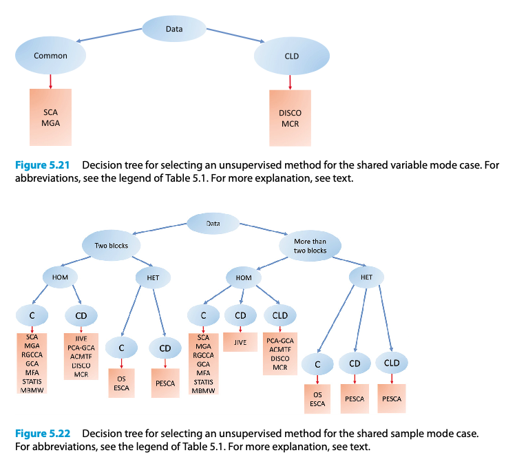
Shared Variable Mode

The chapter begins by examining methods in the shared variable mode, with a specific focus on isolating only common variations such as Simultaneous Component Analysis (SCA), which integrates data from multiple sources to find common patterns. It also addresses more complex structures that include both common and distinct variations, employing methods like Distinct and Common Components Analysis and Multivariate Curve Resolution to dissect the unique and shared signals within the data.

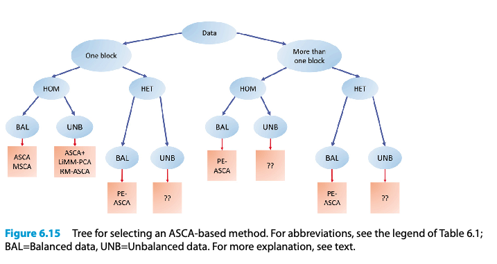
Shared Sample Mode

In the shared sample mode, the discussion shifts towards methods designed to handle data structures where samples are shared across different datasets but the variables may differ. Techniques like SUM-PCA and Multiple Factor Analysis provide tools for extracting common information across these shared samples. The chapter further explores the integration of these methods with statistical techniques like Generalised Canonical Analysis and Regularised Generalised Canonical Correlation Analysis, enhancing their ability to deal with various data complexities including high-dimensionality and under-determined systems. Exponential Family SCA and Optimal-scaling are discussed for their ability to adapt the component analysis to different scales and data distributions.

Advanced Topics

The latter sections of the chapter address more advanced topics, such as Joint and Individual Variation Explained (JIVE) for parsing out distinct and shared information across multiple datasets, and Advanced Coupled Matrix and Tensor Factorisation, which extend these concepts into higher-dimensional data. Penalised-ESCA and further Multivariate Curve Resolution approaches are introduced for dealing with extremely heterogeneous data.

Framework and Methodological Considerations

A generic framework for simultaneous unsupervised methods is outlined, providing a structured approach to applying these diverse methodologies across different types of multiblock data scenarios. This framework helps in identifying the appropriate methodological adjustments needed for specific data characteristics and analysis goals.

Concluding Thoughts

The chapter concludes with a synthesis of the discussed methods, offering recommendations based on the complexities and specific requirements of various data analysis scenarios. Open issues in the field are highlighted, pointing to areas where further research and development are needed to advance the capabilities of unsupervised multiblock data analysis.

Alternative Unsupervised Methods (chapter 9)

9.i General Introduction

This chapter explores some unsupervised methods that are less commonly used than those highlighted in Chapter 5. This does not necessarily indicate that they are less useful, but rather that some are relatively new and their full potential is still being evaluated. We will cover methods that focus on identifying common variation as well as those that can differentiate between common, local, and distinct variations. The methods discussed will apply to data situations with a shared variable mode, a shared sample mode, and scenarios where both modes are shared. We will examine approaches suitable for both homogeneous and heterogeneous data fusion. Throughout this chapter, we will assume that data blocks are column-centred unless stated otherwise, and the default norm used for vectors and matrices will be the Frobenius norm.

9.ii Relationship to the General Framework

This section provides a brief overview of the unsupervised methods discussed in this chapter as outlined in Table 10.1. The table illustrates a diverse range of methods based on different foundational principles. Most methods operate simultaneously and are model-based, including those based on factor analysis models that incorporate penalties (such as BIBFA, GFA, MOFA, and GAS) and are capable of handling heterogeneous data. The representation method (RM) provides a unique approach through three-way models of specially constructed data representations. Other methods discussed include generalizations of SVD (GSVD) and methods based on copulas (XPCA). This diversity showcases the rich variety of data science approaches available to address similar problems across different fields.

9.1 Shared Variable Mode

In scenarios involving a shared variable mode, we explore methods that can distinguish between common and distinct components. One such method is the generalized singular value decomposition (GSVD), also known as quotient SVD (QSVD), which has been developed over the years (Van Loan, 1976; Paige and Saunders, 1981; De Moor and Zha, 1991). GSVD is an eigenvalue-based technique for separating common from distinct components in shared variable contexts.

Generalised SVD

For two data blocks, the GSVD model is formulated as follows: \(X_1 = X̃_1 + E_1 = T_1 D_1 P^T + E_1\) \(X_2 = X̃_2 + E_2 = T_2 D_2 P^T + E_2\) Here, (X̃_m) represents the data filtered through an SCA model applied to the concatenated matrix ([X = [X_1^T|X_2^T]^T]). The matrices (T_m) are orthonormal (i.e., (T_m^T T_m = I)), and (P) is a full-rank matrix of common loadings, which are not necessarily orthonormal. The matrix (D_m) is diagonal, and the constraint (D_1 + D_2 = I) allows the generalised singular values to be categorized into three groups based on their significance in each block, which aids in distinguishing between common and distinct components.

The model structure is such that: \(X_1 = T_{11} D_{11} P_{t1} + T_{12} D_{12} P_{t2} + T_{13} D_{13} P_{t3} + E_1\) \(X_2 = T_{21} D_{21} P_{t1} + T_{22} D_{22} P_{t2} + T_{23} D_{23} P_{t3} + E_2\) The matrices (D_{11}) and (D_{22}) represent distinct components for (X_1) and (X_2), respectively, while (D_{13}) and (D_{23}) indicate the common components. Ideally, the matrices (D_{12}) and (D_{21}) should contain small values, indicating minimal ‘spill-over’ between the distinct and common components.

This method has been applied in various fields, including gene-expression analysis, and has been extended to handle more than two data blocks, allowing for the detection of common, local, and distinct components across multiple blocks. However, determining these components in the context of multiple blocks is complex and requires careful analysis.

9.2 Shared Sample Mode

9.2.1 Only Common Variation

9.2.1.1 DIABLO

A method used in bioinformatics for multiblock data analysis is called Data Integration Analysis for Biomarker discovery using a Latent component method for Omics studies, DIABLO for short. This method relies strongly on the RGCCA method (see Section 5.2.1.4) and has been implemented in a sparse version (Singh et al., 2019). The model formulation is: \(\max \sum_{m,m'=1}^M c_{m,m'} \text{corr}(X_m w_m, X_{m'} w_{m'}) \text{ s.t. } \|w_m\|_2 = 1, \|w_{m'}\|_1 < \lambda_{m'}\) where (c_{m,m’}) indicates connected blocks, components (t_m = X_m w_m) are calculated, (\lambda_m > 0) are user-set penalties, ensuring ( |w_{m’}|1 < \lambda{m’} ) as a lasso-type penalty. Deflation is performed by ( X_{m,\text{new}} = X_m - t_m w_{m’}^T ). This model, similar to RGCCA, uses deflation not trivial to apply (also see Section 2.8). An example of DIABLO is given in Elaboration 9.1, demonstrating a maximization of correlations across three data blocks, generalizing canonical correlation to multiple blocks.

9.2.1.2 Generalised Coupled Tensor Factorisation

Generalised coupled tensor factorisation (GCTF) (Yılmaz et al., 2011) extends coupled matrix tensor factorisation (CMTF) to heterogeneous data using exponential dispersion models (Jørgensen, 1992). It involves minimizing: \(\min \sum_{m=1}^M v_m d_m [X_m - X_m(\theta, \theta_m)]\) with (d_m) as a divergence measure, (\theta) and (\theta_m) as common and block-specific parameters, respectively, and (v_m) as weights. This method is applicable in a Bayesian framework for learning weights (Şimşekli et al., 2013), representing a generalization of GSCA and ESCA models (see Section 5.2.1.5).

9.2.1.3 Representation Matrices

Representation matrices encode variables differently in multivariate analysis, useful for handling diverse data types and measurement scales. Originally termed quantification matrices, these matrices facilitate variable associations analysis. Representation matrices for ratio-, interval-, and ordinal-scaled variables transform variable measurements into forms suitable for generating familiar associations like Pearson and Spearman correlations using: \(q_{jk} = \frac{2 \text{tr}(S^T_j S_k)}{\text{tr}(S^T_j S_j) + \text{tr}(S^T_k S_k)}\) For nominal-scaled variables, square matrices based on indicator matrices are used, particularly effective for categorical data, giving rise to known correlation measures like T2 coefficient (Tschuprow, 1939).

9.2.1.4 Extended PCA

Extended PCA (XPCA) (Anderson-Bergman et al., 2018) employs copulas to handle J-dimensional distributions comprising diverse marginal distributions using a Gaussian copula for PCA. This method integrates empirical distributions estimated from heterogeneous data, offering potential applications in natural and life sciences.

9.2.2 Common, Local, and Distinct Variation

For a shared sample mode, several methods exist to separate common, local, and distinct components, applicable to both homogeneous and heterogeneous data.

9.2.2.1 Generalised SVD

Generalised SVD (GSVD) extends the approach used in shared variable modes to shared sample modes by focusing on consensus scores (T) rather than loadings. For two data blocks X1 (I × J1) and X2 (I × J2): \(X1 = \tilde{X}_1 + E1 = TD1P^T_1 + E1\) \(X2 = \tilde{X}_2 + E2 = TD2P^T_2 + E2\) where (\tilde{X}_m) are SCA-filtered data, T is a full-rank matrix, (P^T_m P_m = I), and (D_1 + D_2 = I). The elements of (D_m) categorize into distinct parts for X1 and X2, and a common part reflected in both X1 and X2 through consensus scores (T1, T2, T3) and respective loadings. An extension of GSVD for more than two data blocks exists (Ponnapalli et al., 2011) but integrating local components remains complex, discussed in Section 11.5.2.

9.2.2.2 Structural Learning and Integrative Decomposition

Structural Learning and Integrative Decomposition (SLIDE) (Gaynanova and Li, 2019), similar to PESCA, imposes group penalties on loading matrices to discover the structure of common, local, and distinct components across data blocks. Starting with an SCA model: \(X1 = TP^T_1 + E1, X2 = TP^T_2 + E2, X3 = TP^T_3 + E3\) After fitting, loading matrices might show patterns such as: \(P1 = [xx00xx], P2 = [xxx000], P3 = [xxxx00]\) indicating components’ relevance across blocks: first two are common, third is local between blocks 2 and 3, and the last are distinct. SLIDE determines the structure of components through penalisation, allowing a re-fit with these identified structures. The method’s uniqueness relies on the same principles as JIVE (Section 5.2.2.1), with variations in group penalties proposed (Van Deun et al., 2011).

9.2.2.3 Bayesian Inter-battery Factor Analysis

Bayesian Inter-battery Factor Analysis (BIBFA) (Klami et al., 2013) builds on Tucker’s inter-battery factor analysis (1958) and its probabilistic counterpart (Browne, 1979). BIBFA separates the common and distinct parts of two data blocks: \(t \sim N(0, I), \quad t_m \sim N(0, I), \quad x_m \sim N(P_m C t + P_m D t_m, \Sigma_m)\) where (P_m) are loadings, (t, t_m) are scores with t representing consensus scores. BIBFA redefines this model in a Bayesian framework with structured priors to determine component numbers and structural models. Its applications include genomics and analytical chemistry (Acar et al., 2015), demonstrating its utility in decomposing complex data into meaningful components, though setting appropriate priors remains crucial for model performance.

These methods collectively address the challenges of multiblock data analysis by delineating shared and unique variance components across various data types, enhancing interpretability and applicative value in diverse scientific domains.

9.2.2.4 Group Factor Analysis

Group Factor Analysis (GFA) is a machine learning method that extends Bayesian Inter-battery Factor Analysis (BIBFA). It begins with a factor analysis model: \(X = TP^T + E\) Assuming (X) is the concatenation of ([X_1 | \ldots | X_M]), the GFA model is expressed as: \([X_1 | \ldots | X_M] = T[P_1 | \ldots | P_M]^T + [E_1 | \ldots | E_M]\) This setup is similar to the SLIDE model but uses a fully stochastic model where the latent variables (T) are Gaussian distributed, an assumption significant for data with inherent structural relationships, such as experimental designs in the natural and life sciences. GFA allows for independent and normally distributed residuals with potentially differing variances across blocks. It applies Bayesian maximum-likelihood estimation with a group-wise ARD prior for identifying common, local, and distinct components. Reported applications include genomics and fMRI studies (Virtanen et al., 2012).

9.2.2.5 OnPLS

OnPLS, an extension of O2PLS, focuses on identifying common and distinct components across multiple data blocks. Initially developed for two data blocks with shared sample modes, the model for two blocks, (X_1) and (X_2), is structured as: \(X_1 = T_1C P_{t1C} + T_1D P_{t1D} + E_1 = X_1C + X_1D + E_1\) \(X_2 = T_2C P_{t2C} + T_2D P_{t2D} + E_2 = X_2C + X_2D + E_1\) Where (T_1DP_{t1D}) and (T_2DP_{t2D}) can be seen as distinct components, previously referred to as structural noise. OnPLS generalizes this structure for multiple blocks, effectively parsing data into components that are either shared, local to specific pairs of datasets, or unique to individual datasets. This model has been used in various omics and metabolomics studies, demonstrating its utility in complex data integration scenarios (Löfstedt and Trygg, 2011).

9.2.2.6 Generalised Association Study

The Generalised Association Study (GAS) integrates features from JIVE with extensions to handle heterogeneous data using exponential family distributions. The model posits: \(\Theta_1 = 1 \mu_{t1} + T C P_{t1C} + T_1D P_{t1D}\) \(\Theta_2 = 1 \mu_{t2} + T C P_{t2C} + T_2D P_{t2D}\) This model structure is similar to JIVE but includes additional constraints for identifiability and assumes pre-determined dimensionalities for matrices (T_C), (T_1D), and (T_2D). GAS estimates model parameters using a block-descent algorithm within a GLM framework, addressing the distinct challenges of handling data with different distributions (Li and Gaynanova, 2018).

9.2.2.7 Multi-Omics Factor Analysis

Multi-omics Factor Analysis (MOFA) is a Bayesian model that extends BIBFA and GFA to accommodate heterogeneous data from multiple sources, such as different omics technologies. It employs: \(X_m = T P_{tm} + E_m; \quad m = 1, \ldots, M\) Where (T) includes all latent variables (common, local, distinct). MOFA uses ARD and spike-and-slab priors to enforce different sparsity levels across the factors, suitable for datasets with varying degrees of underlying structure and noise levels. Its complex Bayesian framework requires robust statistical knowledge for effective application. MOFA’s ability to learn the structure of loadings (P) from data distinguishes it from models requiring a priori structure specifications, like DISCO models (Argelaguet et al., 2018).

The example provided for MOFA and PESCA illustrates the practical applications of these models in understanding complex relationships in chronic lymphocytic leukaemia data, highlighting the flexibility and depth of insights achievable through advanced multiblock data analysis methods.

9.3 Two Shared Modes and Only Common Variation

When datasets possess two shared modes, special analytical methods are required. This typically involves the same set of samples and variables measured across different occasions, demanding techniques that can address the complexities of repeated measurements. The nature of the data and the specific research questions posed dictate the choice of method.

9.3.1 Generalised Procrustes Analysis (GPA)

In contexts such as sensory analysis where different assessors evaluate the same products using the same sensory characteristics, there is a need to achieve consensus among assessors. Generalised Procrustes Analysis (GPA) is well-suited for this purpose. GPA aims to align the configurations of samples across multiple blocks of data (e.g., different assessors) as closely as possible in terms of translation, dilation, and rotation. Column-centring each data block handles translation, while optimal scaling factors and rotation matrices ((\lambda_m)s and (Q_m)s) are used to manage dilation and rotation, minimizing the Frobenius norm of the differences between each block and a consensus configuration (V). This consensus can then be analyzed further, typically with principal component analysis (PCA) to understand the variance and similarities across blocks. GPA’s versatility extends beyond sensory analysis to fields like genomics, indicating its broad applicability in multidisciplinary research.

9.3.2 Three-way Methods

For datasets that can be structured into three-dimensional arrays (three-way data), methods like PARAFAC (Parallel Factor Analysis) and Tucker3 models provide powerful tools for decomposition. These methods are particularly relevant for chemical data measured through techniques like excitation-emission fluorescence spectroscopy, where the goal is to estimate underlying chemical concentrations:

• PARAFAC: Simplifies the analysis by decomposing a three-way array into three matrices corresponding to each mode, linked by a Khatri-Rao product. It assumes a simple structure where each component is linked to only one factor per mode, facilitating interpretation but potentially limiting flexibility.

• Tucker3: Offers a more general form of three-way decomposition, utilizing a core array that interacts with matrices corresponding to each mode. This method can adapt to more complex variations in data structures, accommodating different numbers of components per mode.

These three-way methods extend the concept of PCA to multidimensional data, effectively capturing the inherent structure and correlations within such datasets. Their applications range from analytical chemistry to psychometrics and social sciences, reflecting their adaptability and power in extracting meaningful information from complex data structures.

9.4 Conclusions and Recommendations

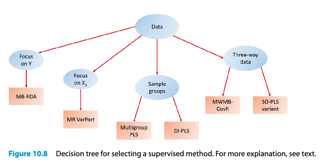
This chapter presents a variety of unsupervised multiblock methods, ranging from GSVD for shared variables to GPA and three-way methods like PARAFAC and Tucker for datasets with shared samples and variables. The choice of method depends on several factors:

• Shared Modes: Whether the dataset involves shared variables, samples, or both.
• Number of Blocks: The complexity and number of data blocks involved.
• Data Homogeneity: Whether the data are homogeneous or heterogeneous.
• Need for Differentiation: Whether there is a need to differentiate between common, local, and distinct components.

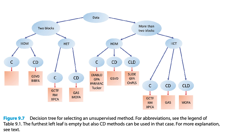
For instance, if the dataset consists of more than two blocks of homogeneous data and requires parsing out common, local, and distinct components, methods like SLIDE, GFA, and OnPLS are suitable choices. SLIDE and GFA are more similar to each other, focusing on simultaneous analysis, whereas OnPLS adopts a sequential approach to component extraction.

9.4.1 Open Issues

Despite the strengths of the methods discussed, there are several open issues:

• Complexity of Methodology: The advanced statistical techniques, such as Bayesian estimation and the use of penalties, require significant expertise and careful tuning.
• Properties of Estimates: The stability and identifiability of the estimated parameters under various conditions remain areas of ongoing research.

These challenges underscore the need for continued development and refinement in unsupervised multiblock data analysis techniques, ensuring their applicability and effectiveness in addressing complex, real-world data analysis scenarios.

Decision trees

Matrix correlation methods

Unsupervised methods for the shared variable mode case and the shared sample mode case

ASCA-based methods

Alternative unsupervised method

Selecting a supervised method

Method list

Chapter 5: Unsupervised Methods in Selected Methods for Unsupervised and Supervised Topologies

1. Simultaneous Component Analysis (SCA) - No specific citation provided.
2. Distinct and Common Components Analysis (DCCA) - No specific citation provided.
3. Multivariate Curve Resolution (MCR) - No specific citation provided.
4. SUM-PCA - No specific citation provided.
5. Multiple Factor Analysis (MFA) - No specific citation provided.
6. Generalised Canonical Analysis (GCA) - No specific citation provided.
7. Regularised Generalised Canonical Correlation Analysis (RGCCA) - No specific citation provided.
8. Exponential Family SCA (ESCA) - No specific citation provided.
9. Optimal-scaling (Optimal-SCA) - No specific citation provided.
10. Joint and Individual Variation Explained (JIVE) - No specific citation provided.
11. Advanced Coupled Matrix and Tensor Factorisation (ACMTF) - No specific citation provided.
12. Penalised-ESCA (P-ESCA) - No specific citation provided.

Chapter 9: Alternative Unsupervised Methods

1. Generalised Singular Value Decomposition (GSVD) also known as Quotient SVD (QSVD)
   • Van Loan, 1976; Paige and Saunders, 1981; De Moor and Zha, 1991.
2. Data Integration Analysis for Biomarker discovery using a Latent component method for Omics studies (DIABLO)
   • Singh et al., 2019.
3. Generalised Coupled Tensor Factorisation (GCTF)
   • Yılmaz et al., 2011; Şimşekli et al., 2013.
4. Extended PCA (XPCA)
   • Anderson-Bergman et al., 2018.
5. Structural Learning and Integrative Decomposition (SLIDE)
   • Gaynanova and Li, 2019.
6. Bayesian Inter-battery Factor Analysis (BIBFA)
   • Klami et al., 2013.
7. Group Factor Analysis (GFA)
   • Virtanen et al., 2012.
8. Orthogonal Projections to Latent Structures (OnPLS)
   • Löfstedt and Trygg, 2011.
9. Generalised Association Study (GAS)
   • Li and Gaynanova, 2018.
10. Multi-Omics Factor Analysis (MOFA)
    • Argelaguet et al., 2018.
11. Generalised Procrustes Analysis (GPA)
    • No specific citation provided.
12. Parallel Factor Analysis (PARAFAC)
    • No specific citation provided.
13. Tucker3 Model
    • No specific citation provided.