Causal inference stats Pearl review
Last update: 20250101
This document is based on [1] “J. Pearl, “Causal inference in statistics: An overview,” Statistics Surveys, 2009, link to pdf. Here is a link to the author’s homepage where you will find the key work highlighted. The complete textbook is [2] “Causality - Models, Reasoning, and Inference”, Second edition, Judea Pearl, link to author page. The same topics are introduced for a general audience in [3] “The Book of Why”, Judea Pearl and Dana Mackenzie, 2018, link to Wikipedia.
This topic is widely ignored. The techincal papers are sometimes verbose and opinionated and thus are difficult to read. An alternative approach is to read the general audience introduction (link 3 above) followed by hands-on work as demonstrated in the tutorial page on causal inference in R.
Introduction
Background: The field of causal inference has advanced significantly, driven by developments in:
- Nonparametric structural equations.
- Graphical models.
- Integration of counterfactual and graphical methods.
Importance: These advances are crucial for empirical sciences to address causal questions in health, social, and behavioral sciences.
Objective: To summarize key advances in causal inference and illustrate their application in empirical research.
From Associational to Causal Analysis: Distinctions and Barriers
2.1 Basic Distinction:
- Statistical Analysis: Infers parameters from a distribution to describe static conditions.
- Causal Analysis: Aims to understand data generation processes, enabling predictions about changes due to interventions or external factors.
- Key Principle: Associations cannot substantiate causal claims; causal analysis requires specific causal assumptions.
2.2 Formulating the Distinction:
- Associational Concepts: Defined by relationships within a joint distribution (e.g., correlation, regression).
- Causal Concepts: Involve relationships that extend beyond observable distributions (e.g., randomization, effect, confounding).
2.3 Ramifications:
- Associational vs. Causal: Confounding, often misconstrued as associational, is inherently causal as it involves discrepancies between observed associations and those under experimental conditions.
- Notational Challenges: Traditional statistical methods and language are insufficient for expressing causal relationships.
2.4 Barrier of Untested Assumptions:
- Associational assumptions are potentially testable; causal assumptions are not without experimental control.
- The clarity of causal assumptions invites scrutiny and requires a shift in how assumptions are conceptualized and communicated.
2.5 New Notation:
- Introduction of specific causal notation is necessary to clearly distinguish between statistical associations and causal relationships.
- Counterfactual notation (e.g., \(Y_x(u)\) or \(P(Y=y \mid \text{do}(X=x))\)) helps express causal concepts that cannot be captured by traditional probability calculus.
The Language of Diagrams and Structural Equations
3.1 Linear Structural Equation Models
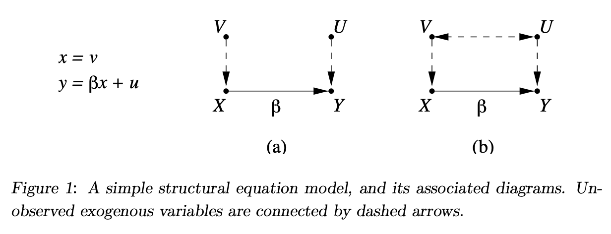
Historical context: Wright (1921) combined equations and diagrams to illustrate causal relationships, e.g., disease (X) causing a symptom (Y): \(y = \beta x + u\) Equation (3.1) illustrates the level of disease (x) influencing the level of symptom (y) with u representing external factors.
Path diagrams: Diagrams clarify causal directions, preventing misinterpretations of equations like reversing (3.1) to suggest symptoms cause diseases.
Model interpretation: In path diagrams, causal influence is indicated by arrows, with their absence denoting no direct causal effect. The model includes exogenous variables (U, V) representing unexplained factors influencing endogenous variables (X, Y).
3.2 From Linear to Nonparametric Models
Evolution of Structural Equation Modeling (SEM): Originally developed for linear relationships, SEM has been extended to nonparametric and nonlinear models.
Reconceptualizing effect: Effects in SEM are redefined as general capacities to transmit changes among variables, beyond algebraic coefficients.
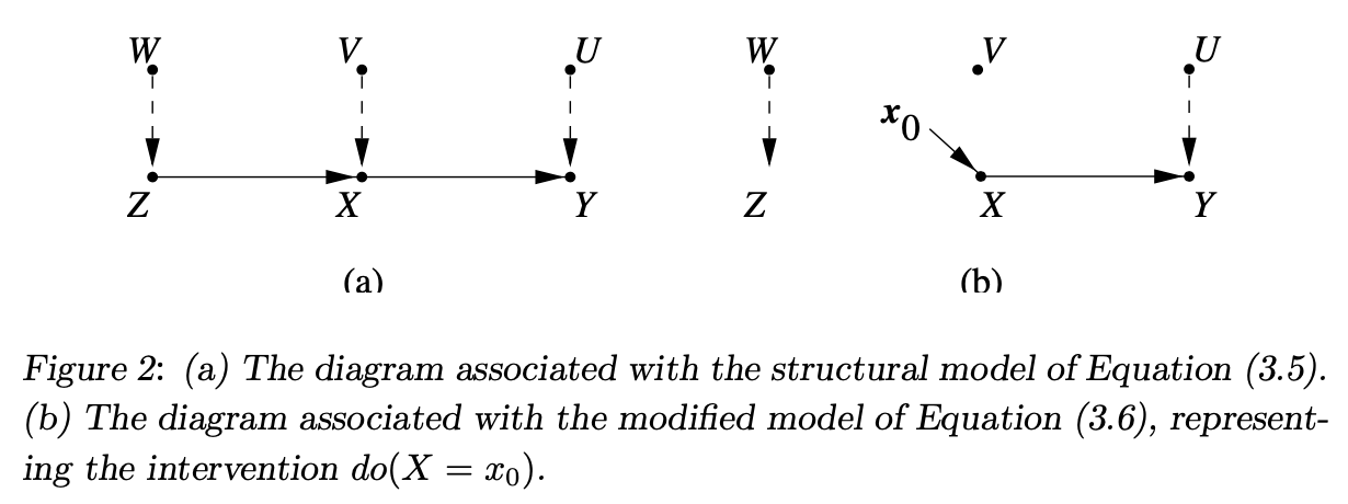
Nonparametric SEM: The new approach uses structural equations to simulate hypothetical interventions: \(z = f_Z(w)\) \(x = f_X(z, v)\) \(y = f_Y(x, u)\) These functions assume that variables are structurally autonomous, invariant to changes in other equations’ forms.
Intervention simulation: The “do” operator (do(x)) represents interventions by setting variables to constants in models, affecting the distribution of other variables: \(x = x_0\) This changes the joint distribution to reflect controlled conditions, providing insights into treatment effects: \(E(Y|do(x'0)) - E(Y|do(x0))\) Equation (3.7) calculates the difference in expected outcomes under different treatment conditions.
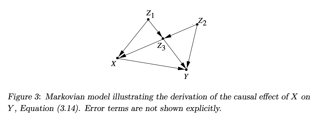
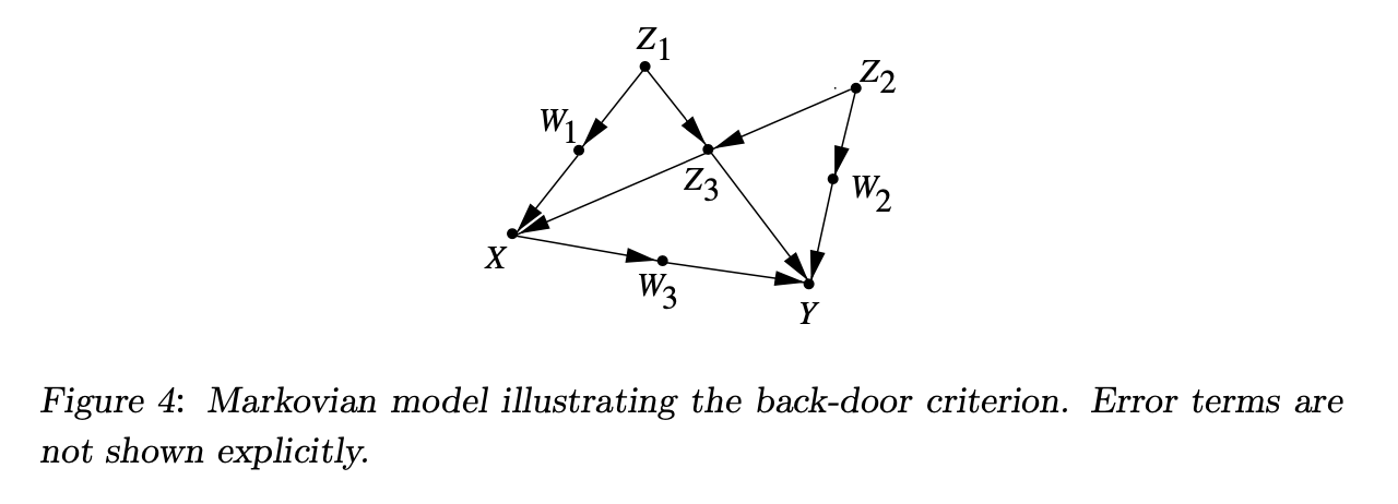
Identifiability and Markovian models: Identification in causal analysis is feasible under Markovian conditions, where: \(P(v1, v2, ..., vn) = \prod P(vi|pai)\) Equation (3.9) expresses the joint distribution as a product of conditional distributions determined by the graph structure.
Truncated factorization: After interventions, distributions are re-factorized to exclude affected variables: \(P(v1, v2, ..., vk|do(x0)) = \prod_{i|Vi \notin X} P(vi|pai)|_{x=x0}\) Equation (3.11) reflects distributions post-intervention, essential for deriving causal effects from observational data.
These sections outline how causal relationships are modeled using equations and diagrams, and how these models adapt to non-linear and nonparametric forms to estimate effects of interventions in complex systems.
3.3 Counterfactual Analysis in Structural Models
Conceptual Framework: Counterfactual analysis explores causal relationships not expressible by experimental setups or \(P(y|do(x))\), using counterfactual notation \(Y_x(u) = y\) to examine potential outcomes in hypothetical scenarios.
Interpretation of Counterfactuals: The approach modifies the original model by replacing variables with constants to reflect hypothetical conditions, thus formalizing counterfactual queries within structural equation models.
For example, in a modified model: \(Y_{x_0}(u,v,w) = Y_{x_0}(u) = f_Y(x_0,u)\) This represents the potential response \(Y\) to a hypothetical treatment \(x_0\).
Attribution and Susceptibility: Counterfactuals allow calculation of effects like change due to treatment, expressed as: \(Y_{x_1} = \beta(x_1 - x_0) + y_0\) This signifies how the outcome \(Y\) would change if \(X\) were \(x_1\) instead of \(x_0\).
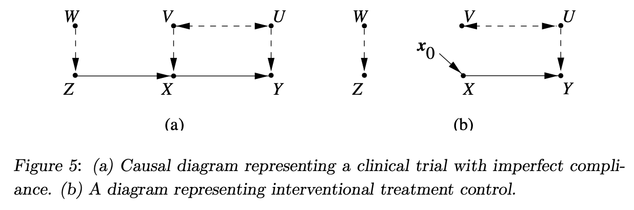
3.4 An Example: Non-Compliance in Clinical Trials
Formulating the Assumptions
Model Setup: Considers a clinical trial model with variables \(Z\) (randomized treatment assignment), \(X\) (treatment received), and \(Y\) (response), influenced by unobserved factors \(U\) and \(V\).
Diagram of a Clinical Trial with Imperfect Compliance:
- Figure 5(a): Shows the causal relationships, including compliance and response pathways.
- Exclusion Restriction: Assumes \(Z\) influences \(Y\) only through \(X\), not directly.
- Randomization Assumption: \(Z\) is independent of \(U\) and \(V\), ensuring no common cause affecting both.
Estimating Causal Effects
Non-identifiability: The causal effect of treatment on outcome is not identifiable directly due to unobserved confounders \(V\) and \(U\), without further assumptions.
Instrumental Variables Approach: Linear case: Uses correlation to determine causal effect, with: \(\beta = \frac{Cov(Z, Y)}{Cov(Z, X)}\) Equation (3.22) shows the use of instrumental variables to estimate causal effects when direct measurement or control of confounders is not possible.
Bounding Causal Effects
Bounds Determination: When exact causal effects can’t be identified, the analysis seeks to establish bounds on these effects based on observed data.
Instrumental Inequality: Ensures any variable \(Z\) serves as an instrument only if it meets specific conditions, reflected by the inequality: \(\max \left[ \max P(x, y|z) \right] \leq 1\) Equation (3.25) imposes constraints on the observed distribution to maintain the validity of the instrumental assumptions.
Testable Implications
Detection of Violations: Specific inequalities derived from the model help detect violations of assumptions regarding the absence of direct effects of \(Z\) on \(Y\) or hidden biases.
Non-compliance and Side Effects: The model assesses non-compliance impacts and side effects through observational inequalities, aiding in understanding the limitations and robustness of causal inferences in clinical trials with partial compliance.
4 The Language of Potential Outcomes and Counterfactuals
4.1 Formulating Assumptions
- Concept: The potential outcome framework utilises Yx(u), representing the outcome Y for unit u if X were x, handling this as a random variable Yx.
- Axiomatic Framework: The framework postulates a comprehensive probability function covering both real and hypothetical events.
- Consistency Constraints: It asserts that if X equals x, then Yx must match the observed Y. \(X = x \Rightarrow Yx = Y\) Equation (4.1) aligns the potential outcome with the observed outcome when the intervention aligns with the actual treatment.
4.2 Performing Inferences
Conditional Ignorability: Assumes conditional independence of Yx and X given Z (Yx ⊥ X | Z), allowing for straightforward calculation of causal effects using potential outcomes: \(P(Yx = y) = \sum_z P(Y = y | X = x, z)P(z)\) Equation (4.5) effectively aligns with standard covariate adjustment formulas, leveraging observed data to infer counterfactual scenarios.
4.3 Combining Graphs and Algebra
- Translation of Assumptions: Graphs convey causal assumptions, translating into counterfactual notation to express and verify causal relationships.
- Parent Sets and Exclusion Restrictions: Define relationships and independence among variables, using the structure to ensure interventions only affect relevant pathways.
- Graph-Assisted Analysis: Graphs help validate and explore dependencies and independencies essential for deriving causal inferences, using criteria like d-separation for testing conditional independencies.
5 Conclusions
Structural Equation Models (SEMs): Presented as a formal language for articulating causal assumptions, enabling clear representation of complex causal relationships.
Integration of Methods: Combining SEMs with potential outcomes enriches the statistical toolkit, allowing for robust empirical research through a unified approach that encapsulates randomization, intervention, effects, and confounding in a coherent framework.
This synthesis of graphical models and algebraic potential outcomes facilitates a deeper understanding and application of causal inference techniques in statistical research, enhancing both theoretical and practical approaches to exploring causality in complex systems.