Last update: 20250307
Table of contents
Multiblock Data Fusion Options
This document outlines three levels of data fusion methods:
High-level data fusion
- Approach: integration of outcomes from individual models.
- Key features:
- treat each data block separately
- combine summary statistics or predictions
- utilise ensemble learning or voting schemes
- Use case: when joint interpretation of biomarker patterns or decision fusion is desired
Mid-level data fusion
- Approach: extract and integrate features from each data block.
- Key features:
- dimensionality reduction methods (e.g. PCA, PLS) to obtain scores
- two-step procedure:
- middle-up: reduce dimensions then concatenate scores
- middle-down: select key variables then concatenate subsets
- Use case: when intermediate patterns or characteristics are needed for further analysis
Low-level data fusion
- Approach: direct integration of raw signals or data.
- Key features:
- analyse relationships across data blocks
- factor analysis or multiblock modelling to create components
- optimise for both within-block representation and between-block correlation
- Use case: when it is necessary to capture detailed inter-variable and inter-block relationships
Final notes
Matrix factorisation
Below is an example of how individual contributions from each data block can combine into a global factor for three factors (F_1), (F_2), and (F_3):
\[F_1 = X_1^1 w_1^1 + X_2^1 w_2^1 + \dots + X_n^1 w_n^1\] \[F_2 = X_1^2 w_1^2 + X_2^2 w_2^2 + \dots + X_n^2 w_n^2\] \[F_3 = X_1^3 w_1^3 + X_2^3 w_2^3 + \dots + X_n^3 w_n^3\]The objective is often to maximise the overall covariance across blocks:
\[\max \sum_{j,k} \operatorname{cov}\bigl(X_j^m w_j^m,\; X_k^m w_k^m\bigr)\]Correlation, variance and covariance
Correlation quantifies the relationship between two variables. This principle is extended to assess links between entire data blocks:
\[\operatorname{corr}(x,y) = \frac{\operatorname{cov}(x,y)}{\sqrt{\operatorname{var}(x)\,\operatorname{var}(y)}}\]Extracting structures from data
Data components are linear combinations of original variables. Their relationships can be compared using:
\[\operatorname{cov}^2\bigl(X_j w_j,\; X_k w_k\bigr) = \operatorname{var}(X_j w_j)\,\operatorname{corr}^2\bigl(X_j w_j,\; X_k w_k\bigr)\,\operatorname{var}(X_k w_k)\]The RV coefficient is an alternative that compares sample configurations across matrices, even when variable counts differ.
Methods like partial least squares (PLS) determine the first latent variables (t_1) and (u_1) for two data blocks by maximising their covariance.
Low-level horizontal multiblock analysis
This approach integrates multiple data blocks sharing the same observations. It can be considered at two levels:
block level (local): \(w'X_1,\quad w'X_2,\quad w'X_3\)
super level (global): global scores combine the individual block contributions, for example: \(tX_s,\quad w^T,\quad qX,\quad uY,\quad Y\)
The super level is constructed based on the chosen model and aims to capture overall patterns.
Methods and criteria to be optimised
Many methods require choosing which variation to prioritise. In practice, covariance is used as a criterion to balance within-block detail and between-block connections.
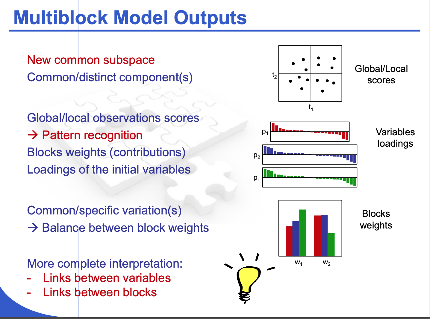
Potential model outputs
- new common subspace: shared latent components revealing global patterns
- common/distinct components: factors separating shared structure from block-specific variation
- pattern recognition: improved detection of meaningful relationships across variables
- global/local observation scores: individual sample scores facilitating both overall and block-level interpretations
- variables loadings: insights into which variables contribute most strongly to each component
- block weights: balancing each block’s influence on the global model
- more complete interpretation: linking variables within each block and across multiple blocks
Slide from SIB training github.